
What to Check Before Tuning a Qdrant Collection
Before you change a setting, decide what better retrieval means for your workload. The right document at rank one, more candidates for a reranker, lower latency, and a smaller memory footprint each favor different settings, so pick your goal first. If your labeled queries can’t detect the improvement you’re chasing, you won’t be able to tell whether a change helped.
Some settings are there to verify your setup, not to tune performance. A sparse vector missing the IDF modifier or a wrong BM25 average length degrades ranking without an error, so any benchmark you run on top of it measures a configuration error. Unindexed vectors are different: Qdrant searches them with an exact scan, which returns valid results, but latency is higher and graph settings such as hnsw_ef have no effect until the index exists. This article shows you how to check each setting and what the expected state looks like.
The Retrieval Pipeline You Are Tuning
Every query first retrieves candidates, then ranks them. In dense-only search, one vector search does both. Hybrid search adds a sparse prefetch for exact terms, then fusion combines the dense and sparse candidate lists. A reranker, if present, scores the top candidates again.
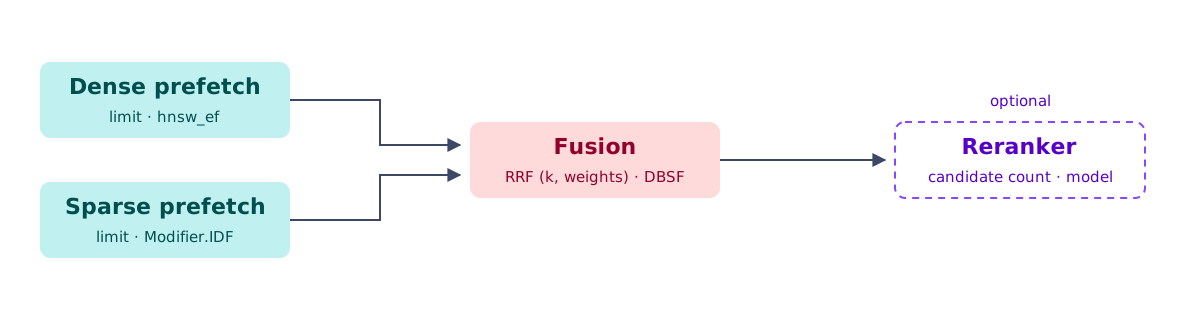
limit and hnsw_ef are its only settings here.If you run dense-only search and exact keywords are missing from results, hybrid search is the first change to test. Tuning hybrid search covers the request shape, what the second prefetch costs, and how to check that fusion beats either prefetch on your labels.
Before you tune:
- Check that indexing has caught up with your data and that every field used in a filter has a payload index. Collection details and payload indexing show what to inspect.
- Build a labeled query set and choose a metric that matches the product experience. A labeled query pairs a real user query with the documents that should be returned. Measuring retrieval relevance walks through the setup.
The Symptom Tells You Where to Start
Start with the failure mode, not the config reference. The table maps each symptom to the first useful check and the article that covers it.
| What You See | First Check | Read Next |
|---|---|---|
| You cannot separate a gain from noise | Build labeled queries, choose a metric, and calculate an interval | This article |
| Relevant documents do not appear | Measure whether candidate depth is limiting recall | Candidate Depth: How Much Retrieval Is Enough? |
| Keywords, identifiers, SKUs, or error codes do not match | Add a sparse prefetch and measure fusion against each prefetch alone | How to Tune Hybrid Search in Qdrant |
| Relevant documents are present but misordered | For hybrid search, tune fusion. If the candidate list needs another ranking stage, test a reranker | How to Tune Hybrid Search in Qdrant, When Is a Reranker Worth It? |
| Results repeat near-duplicates | Test maximal marginal relevance. If chunks from one document fill the page, use grouping | When Is a Reranker Worth It? |
| Search misses its p95 target | Measure the cost of candidate depth before adding another retrieval stage | Candidate Depth: How Much Retrieval Is Enough? |
| The collection no longer fits in RAM | Test memory placement and rescoring | When Your Collection Outgrows RAM |
How to Read These Measurements
The procedure transfers: choose a metric that matches the product experience, compare settings on labeled queries, and validate the winner on fresh queries.
Qdrant’s API and algorithm mechanics carry across collections. The result of a parameter sweep depends on the embedding model, dataset, query mix, filters, index state, shard layout, and deployment. Use each result to choose a test on your own collection, then keep only the settings your labels support.
Silent Settings Can Break Quality
Check the stages you run before tuning anything else. Each prerequisite has an expected state for a given collection and can drift from it without an error. Fix them before you benchmark or compare settings, otherwise you are measuring a configuration error or an unfinished index, not a trade-off.
Dense Search and Indexing
Vectors are indexed Call GET /collections/{collection_name} and compare indexed_vectors_count with points_count. Both are approximate, and their relation depends on the configuration: Qdrant counts each named vector separately, so a collection with one dense and one sparse vector per point can report up to twice points_count. Treat the comparison as a rough signal, not an equality test. A count that stays well below what you expect after ingestion settles, or a status other than green, is what to investigate.
If the indexed count is lower, indexing may still be running, may have stopped, or some segments may be smaller than the default indexing_threshold of 10,000 KB. See the indexing optimizer documentation. Qdrant builds an HNSW graph only after a segment reaches indexing_threshold. Before then, it searches the segment with an exact scan. The results are still correct, but they cost more time per query, and changing hnsw_ef has no effect. Wait for indexing to finish before you measure latency or tune graph settings.
full_scan_threshold Dense and sparse vectors have separate thresholds in different units, so a value copied between them lands nowhere near the intended size. The dense threshold counts kilobytes of vectors in a segment, 10,000 by default. It sends a search to an exact scan instead of the graph when the segment holds fewer vectors than that, or when a filter matches fewer points than that.
The sparse threshold counts vectors, 5,000 by default, and applies only when a filter is present.
Sparse Retrieval
These settings apply whether the collection has thousands of documents or billions.
Modifier.IDF Use this modifier for sparse vectors from BM25 or miniCOIL. Both leave inverse document frequency (IDF) to Qdrant, which computes it per shard for each query term and weights the term by it. SPLADE already includes corpus-level term weighting, so applying the modifier would count rarity twice.
BM25 avg_len Set avg_len to the average number of tokens in the field after BM25 stems words and removes stopwords. BM25 uses this value to adjust for document length. Do not estimate it from raw word counts. In the five datasets tested here, the stemmed count was 15% to 43% lower. The correct values ranged from 35.3 to 151.4, compared with the default of 256. Measure it using the same stemmer and stopword settings as the collection.
Hybrid Search
Fusion placement matters on sharded collections. score_threshold is a risk at any scale when a request moves from single-vector retrieval to fusion.
Fusion placement At the root of the query, fusion runs once, after every shard returns its candidates. Inside a prefetch, fusion runs on each shard. Each shard fuses only its own candidates, and the outer query ranks by those shard-local fused scores. The result changes with shard count and with how points are distributed, and no error tells you it happened. Nested fusion is deliberate when an outer stage rescores its output. On a single-shard collection, both placements produce the same ranking.
score_threshold Use score_threshold only when you have a measured minimum acceptance score for the stage that returns results. A threshold copied from dense-only search is unsafe in a root-level RRF or DBSF query. Qdrant compares it with the fused score, not the dense or sparse score. It can silently truncate the result list or return no results. Validate it on labeled queries, or leave it unset.
Filtered Search
Index every field you filter on. The cost of skipping one grows with collection size and query concurrency.
Payload indexes A healthy collection has a payload index for every field used in its filters. Create these indexes before ingestion. If you add one later, Qdrant does not add the filter-aware HNSW edges automatically. You must rebuild the HNSW index. Qdrant Cloud strict mode rejects queries that filter on unindexed fields. Even with the right indexes, strict filters can reduce recall. What ACORN fixes, and what fixes ACORN measures this effect on one million points.
Change Things in Cost Order
Start with a change that does not rebuild the collection or add a retrieval stage. Move to a higher-cost tier only when the lower-cost options do not address the symptom.
| Tier | What | Applies To | Cost |
|---|---|---|---|
| No New Retrieval Work | Fusion method, RRF k, weights | Hybrid search | Reorders lists you already retrieved. No rebuild or extra retrieval stage |
| Expanded Retrieval | hnsw_ef | Dense search | Increases search breadth and query time |
| Expanded Retrieval | Prefetch limit | Any pipeline with a downstream stage | Retrieves more candidates, increasing query time |
| Expanded Retrieval | full_scan_threshold | Dense search, especially filtered search | Uses exact scans for larger candidate pools, which can increase query time |
| A New Stage | Sparse prefetch | Dense-only search | A second index, a second vector per point, and 0.6 to 1.5 ms of query time on one shard |
| A New Stage | Reranker | Any pipeline | A model call per candidate |
| Rebuild | Embedding model, m | Every collection | Re-indexing the collection. Changing the embedding model also means generating a new vector for every point |
| Rebuild | Quantization | Collections limited by memory | Re-indexing, plus a compressed copy of every vector. Holding ranking quality then depends on rescoring |
Consider a model-level rebuild only when it addresses a measured constraint, since a new embedding model means re-embedding every point. How to choose an embedding model covers that decision. When memory is the constraint, a Matryoshka model’s mrl parameter shortens the vector itself, which is a different trade from compressing it with quantization.
Choose a Metric Before You Tune
Choose the metric before you compare settings, because the metric decides the winner. In our testing, nDCG@10, MRR@10, and Recall@100 each name a different best setting, and Recall@100 disagrees with nDCG@10 on four of five datasets.
nDCG@k rewards relevant results near the top, gives additional credit when labels are graded, and normalizes each query against a perfect ranking. Use it when rank order among several results matters.
MRR@k is the mean of one over the rank of the first relevant result. It asks how fast you got to something good. Use it when a query has one right answer.
Recall@k is the share of all relevant documents that made it into the top k. Use it when you measure a first stage that feeds something else. It is capped per query by the number of relevant documents: a query with 359 relevant documents cannot exceed 0.28 at Recall@100, because only 100 can fit. The average across queries can land higher, because queries with fewer relevant documents are not held to that cap. In our testing, one dataset averages 358.9 relevant documents per query, and its best Recall@100 was 0.3877. Count relevant documents per query before choosing k.
Make Sure Your Labels Can Detect a Gain
Retrieval relevance covers building a labeled set. Its size decides whether any retrieval tuning is visible to you at all.
A labeled set is large enough when it can distinguish the improvement you care about from normal query-to-query variation. Size alone will not save an unrepresentative set. Pull queries across the mix your product sees, including its important query types and filters, and spot-check a sample of the labels yourself.
Every check below takes one score per query for each setting you are comparing. Use the Qdrant request your service already sends. The scoring is the same whether your pipeline runs dense-only search, hybrid fusion, or a reranker.
Scoring starts with the metric itself. dcg sums graded relevance with a discount that grows with rank. ndcg_at_k runs that sum on what came back, then divides it by the same sum over the best ordering the query’s labels allow.
import math


def dcg(gains):
    """Relevance summed with a discount that grows with rank."""
    return sum(gain / math.log2(rank + 2) for rank, gain in enumerate(gains))


def ndcg_at_k(doc_ids, relevance, k=10):
    """One query's ranking against the best ranking its labels allow."""
    returned = [relevance.get(doc_id, 0) for doc_id in doc_ids[:k]]
    ideal = sorted(relevance.values(), reverse=True)[:k]
    return dcg(returned) / dcg(ideal) if any(ideal) else 0.0
Then run your labeled queries through both settings. You write search, which applies one setting to the request your service already sends and returns the points as the server ranked them. Add with_payload=["doc_id"] to that request so every point carries the ID your labels use, or read point.id if your point IDs are already your document IDs. score turns each list into one number, and subtracting the two scores for each query gives the per-query gain.
# Relevance keyed by the document IDs your labels already use.
qrels = {"q1": {"doc-41": 1, "doc-77": 2}}
# Your labeled queries. Each value is what search sends to Qdrant: text or a vector.
queries = {"q1": [...]}
# The one parameter under test, in whatever form your search applies it.
current_setting = {"hnsw_ef": 64}
candidate_setting = {"hnsw_ef": 256}


def search(query_id, query, setting):
    """You write this: your own Qdrant request, with setting applied.

    Return the points in the order the server ranked them, each carrying doc_id.
    """
    raise NotImplementedError


def score(queries, qrels, search, setting):
    """One nDCG@10 per query, for one setting."""
    return {
        query_id: ndcg_at_k(
            [point.payload["doc_id"] for point in search(query_id, query, setting)],
            qrels.get(query_id, {}),
        )
        for query_id, query in queries.items()
    }


candidate = score(queries, qrels, search, candidate_setting)
current = score(queries, qrels, search, current_setting)
per_query_gain = [candidate[q] - current[q] for q in sorted(queries)]
The two calls must differ in exactly one setting. Filters, query shape, and candidate limits stay identical. For MRR@10 and Recall@100, pytrec_eval computes both from the same qrels.
Resample the per-query gains with replacement to estimate how much the average gain would move if you had drawn a different set of queries. The resulting 95% interval shows the range consistent with that sampling variation. If the interval includes zero, your labels cannot establish a quality gain.
import numpy as np

def interval(per_query_gain, resamples=1000, seed=42):
    """95% interval for the mean per-query gain of one setting over another."""
    gains = np.asarray(per_query_gain, dtype=float)
    rng = np.random.default_rng(seed)
    draws = rng.integers(0, len(gains), size=(resamples, len(gains)))
    return np.percentile(gains[draws].mean(axis=1), [2.5, 97.5])
The more labeled queries you evaluate, the more precise the measured gain. Across our datasets, the 95% interval typically extended this far above and below the nDCG@10 gain:
| Labeled Queries | Interval, Either Side of the Gain |
|---|---|
| 25 | 0.047 |
| 50 | 0.035 |
| 100 | 0.025 |
| 200 | 0.018 |
| 300 | 0.015 |
The label count you need depends primarily on effect size and query-to-query variation, not collection size alone.
In our measurements, fusion settings moved nDCG@10 by 0.012 to 0.038, gains from tuning an already-working collection rather than rebuilding the retrieval pipeline.
Fifty labeled queries were enough for the larger gains: the 0.038 gain had an interval excluding zero in 93% of draws, while gains under 0.02 cleared that bar in 7% to 38%. Treat small movement as unresolved until you have the labels to measure it.
Check the Winner on Fresh Queries
A setting selected and evaluated on the same queries will look better than it performs on fresh queries. Split the labeled queries in half: select the winner on one half, then measure its gain on the other. We repeated that split 200 times per dataset.
The selected setting usually transfers. Ranking all 30 settings again on the fresh half, our pick typically landed in the top four, and it fell behind the default in 0% to 6% of splits. The gain does shrink: it retained 67% to 95% of what selection reported, so report the number from the fresh queries.
If you compare separately rebuilt indexes, check top-10 agreement across two builds before you treat a small nDCG@10 difference as a tuning gain. In our clean rebuild test, query sampling moved nDCG@10 more than graph variation did.
Start with One Change
Record the current relevance metric and p95 latency for a representative query set. Choose one low-cost change from the symptom table, validate it on fresh queries, and keep it only if the gain survives. Once you have that baseline, Candidate Depth: How Much Retrieval Is Enough? shows how to test whether retrieval depth is the constraint.
 Ready to try Qdrant?