
Anomaly detection is a thirsting yet challenging task that has numerous use cases across various industries. The complexity results mainly from the fact that the task is data-scarce by definition.
Similarly, anomalies are, again by definition, subject to frequent change, and they may take unexpected forms. For that reason, supervised classification-based approaches are:
- Data-hungry - requiring quite a number of labeled data;
- Expensive - data labeling is an expensive task itself;
- Time-consuming - you would try to obtain what is necessarily scarce;
- Hard to maintain - you would need to re-train the model repeatedly in response to changes in the data distribution.
These are not desirable features if you want to put your model into production in a rapidly-changing environment. And, despite all the mentioned difficulties, they do not necessarily offer superior performance compared to the alternatives. In this post, we will detail the lessons learned from such a use case.
Coffee Beans
Agrivero.ai - is a company making AI-enabled solution for quality control & traceability of green coffee for producers, traders, and roasters. They have collected and labeled more than 30 thousand images of coffee beans with various defects - wet, broken, chipped, or bug-infested samples. This data is used to train a classifier that evaluates crop quality and highlights possible problems.
Anomalies in coffee
We should note that anomalies are very diverse, so the enumeration of all possible anomalies is a challenging task on it’s own. In the course of work, new types of defects appear, and shooting conditions change. Thus, a one-time labeled dataset becomes insufficient.
Let’s find out how metric learning might help to address this challenge.
Metric Learning Approach
In this approach, we aimed to encode images in an n-dimensional vector space and then use learned similarities to label images during the inference.
The simplest way to do this is KNN classification. The algorithm retrieves K-nearest neighbors to a given query vector and assigns a label based on the majority vote.
In production environment kNN classifier could be easily replaced with Qdrant vector search engine.
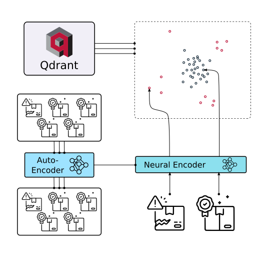
Production deployment
This approach has the following advantages:
- We can benefit from unlabeled data, considering labeling is time-consuming and expensive.
- The relevant metric, e.g., precision or recall, can be tuned according to changing requirements during the inference without re-training.
- Queries labeled with a high score can be added to the KNN classifier on the fly as new data points.
To apply metric learning, we need to have a neural encoder, a model capable of transforming an image into a vector.
Training such an encoder from scratch may require a significant amount of data we might not have. Therefore, we will divide the training into two steps:
The first step is to train the autoencoder, with which we will prepare a model capable of representing the target domain.
The second step is finetuning. Its purpose is to train the model to distinguish the required types of anomalies.
Model training architecture
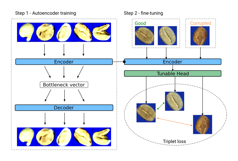
Step 1 - Autoencoder for Unlabeled Data
First, we pretrained a Resnet18-like model in a vanilla autoencoder architecture by leaving the labels aside. Autoencoder is a model architecture composed of an encoder and a decoder, with the latter trying to recreate the original input from the low-dimensional bottleneck output of the former.
There is no intuitive evaluation metric to indicate the performance in this setup, but we can evaluate the success by examining the recreated samples visually.

Example of image reconstruction with Autoencoder
Then we encoded a subset of the data into 128-dimensional vectors by using the encoder, and created a KNN classifier on top of these embeddings and associated labels.
Although the results are promising, we can do even better by finetuning with metric learning.
Step 2 - Finetuning with Metric Learning
We started by selecting 200 labeled samples randomly without replacement.
In this step, The model was composed of the encoder part of the autoencoder with a randomly initialized projection layer stacked on top of it. We applied transfer learning from the frozen encoder and trained only the projection layer with Triplet Loss and an online batch-all triplet mining strategy.
Unfortunately, the model overfitted quickly in this attempt. In the next experiment, we used an online batch-hard strategy with a trick to prevent vector space from collapsing. We will describe our approach in the further articles.
This time it converged smoothly, and our evaluation metrics also improved considerably to match the supervised classification approach.
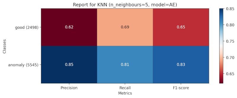
Metrics for the autoencoder model with KNN classifier
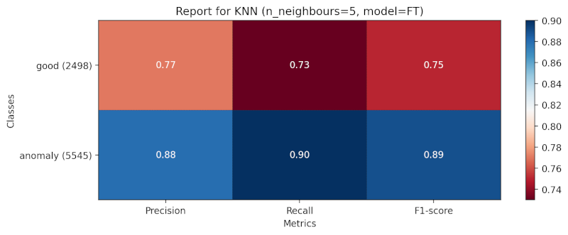
Metrics for the finetuned model with KNN classifier
We repeated this experiment with 500 and 2000 samples, but it showed only a slight improvement. Thus we decided to stick to 200 samples - see below for why.
Supervised Classification Approach
We also wanted to compare our results with the metrics of a traditional supervised classification model. For this purpose, a Resnet50 model was finetuned with ~30k labeled images, made available for training. Surprisingly, the F1 score was around ~0.86.
Please note that we used only 200 labeled samples in the metric learning approach instead of ~30k in the supervised classification approach. These numbers indicate a huge saving with no considerable compromise in the performance.
Conclusion
We obtained results comparable to those of the supervised classification method by using only 0.66% of the labeled data with metric learning. This approach is time-saving and resource-efficient, and that may be improved further. Possible next steps might be:
- Collect more unlabeled data and pretrain a larger autoencoder.
- Obtain high-quality labels for a small number of images instead of tens of thousands for finetuning.
- Use hyperparameter optimization and possibly gradual unfreezing in the finetuning step.
- Use vector search engine to serve Metric Learning in production.
We are actively looking into these, and we will continue to publish our findings in this challenge and other use cases of metric learning.