
Filtered Vector Search: What ACORN Fixes, and What Fixes ACORN
Dylan Couzon & Meina Ghafouri
·August 07, 2026

Filtered vector search breaks when metadata filters turn a healthy nearest-neighbor graph into scattered islands. HNSW’s m parameter controls how many links each point gets. At Qdrant’s default m=16, the one-million-point collection benchmarked in this article averaged about 21 links per node on layer 0. Filter out 96% of the points and fewer than one link per node survives on average, so traversal can get stranded before it reaches the true nearest matches.
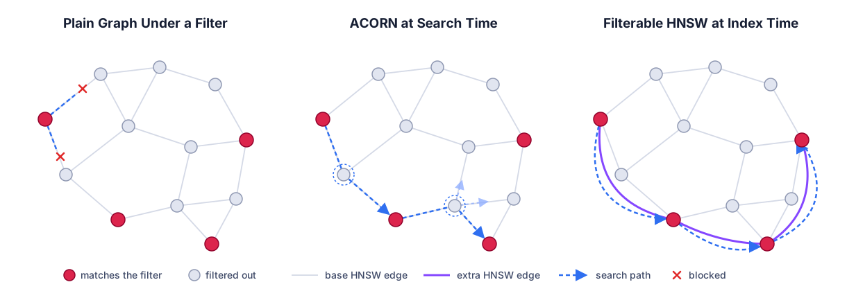
Qdrant repairs that damage in two places. Filterable HNSW adds extra edges at index time; ACORN steps through neighbors of neighbors at search time. Both run on the same collection. ACORN earns its cost where the extra edges don’t reach: values too common to link, AND filters no single field’s edges cover, and payload fields the build skipped silently.
This benchmark runs on a single Qdrant instance and compares four of Qdrant’s own search strategies over four builds.
The Two ACORNs
The ACORN paper (Patel et al., SIGMOD 2024) describes two algorithms. Its headline claim of “2-1,000x higher throughput at a fixed recall” belongs to ACORN-gamma, which expands neighbor lists during index construction at 8.8x to 33.1x plain HNSW’s build time in the paper’s own table.
ACORN-1 is lighter. It builds a standard HNSW graph, then checks neighbors of neighbors at search time where direct neighbors fail the filter. Qdrant implements ACORN-1 as a query parameter you opt into per request, with no index-time changes.
The Graph Qdrant Builds Instead
Filterable HNSW, which our co-founder Andrey Vasnetsov described in 2019, builds the repair into the index. When a payload field, the metadata attached to each point, is indexed, Qdrant adds extra HNSW edges between points that share a value in that field, so a filtered query keeps a connected graph to traverse. Qdrant gives those edges to payload fields at index time, and not every field earns them.
Those edges cost build time. On our one-million-point collection, the HNSW index built in 116 seconds without them and 507 to 652 seconds with them, 4.4x to 5.6x the cost. That range covers two builds at identical settings, so it is build-to-build variance. Both figures are index build time, with ingest excluded.
Qdrant builds those edges per payload field, never per combination, so an AND filter lands on an intersection that no single field’s edges cover. ACORN-1 covers that gap and pays at query time instead of build time. Qdrant’s query planner chooses automatically between ACORN, full scan, retrieval straight from the payload index, and filterable HNSW.
Switch between the three searches to see how each handles the same filter.
The Benchmark
The benchmark runs on one million deep-image-96 vectors, 96-dimensional image embeddings from the ANN-benchmarks suite. Keyword filters match from 20% of the points down to 0.012%. Recall@10 is scored against exact brute force over 500 queries per filter, and latency is mean server-side query time.
We tested four strategies:
- Plain graph: standard HNSW with no extra edges.
- Plain graph + ACORN: the same graph with ACORN forced on.
- Filterable HNSW: the default build with extra edges.
- Planner + ACORN: Qdrant’s default query planner, free to route each query to ACORN, full scan, or the payload index.
Every filter matches one keyword value on a payload field. The collection carries seven such fields, holding 5, 10, or 100 distinct values each.
Most filters are independent of the vectors. The Correlated (10%) row is the easy case, where points that pass the filter also sit near each other in vector space.
Every number in this article was measured on Qdrant v1.18.2, on one laptop-class machine, queried serially. Read the ratios, not the absolute milliseconds. The reproduction kit documents the hardware and the full methodology.
Single Filters: Extra Edges Win
hnsw_ef, shortened to ef in this article, is the number of candidates the search evaluates, so raising it improves recall and slows the query. Selectivity is the fraction of points that pass the filter.
This table compares the first three strategies. full_scan_threshold tells Qdrant when a filtered result set is small enough to scan directly. The value is measured in kilobytes of vector data, and Qdrant skips the HNSW graph when the matching vectors fall below it.
We pinned it low for these three strategies so every query stayed on the graph; Planner + ACORN runs with the default threshold. Each cell shows Recall@10 and mean server-side latency at hnsw_ef=64.
| Filter (selectivity) | Plain graph | Plain graph + ACORN | Filterable HNSW |
|---|---|---|---|
| One keyword (20%) | 62.9% @ 1.6ms | 98.9% @ 4.4ms | 94.8% @ 1.2ms |
| One keyword (10%) | 20.6% @ 1.7ms | 98.1% @ 4.3ms | 99.0% @ 1.1ms |
| One keyword (1%) | 0.1% @ 1.6ms | 67.7% @ 4.7ms | 99.8% @ 1.0ms |
| Correlated (10%) | 88.4% @ 1.7ms | 98.6% @ 3.5ms | 99.0% @ 1.2ms |
The plain graph collapses as filters tighten, and only the correlated filter holds up. ACORN pulls recall back at 2.1x to 2.9x the plain graph’s latency, then stalls on the 1% filter, the weakness the RACORN-1 follow-up paper targets. The one filter ACORN wins, at 20%, runs on a payload field that got no extra edges, and the next section explains why.
Qdrant’s planner chooses among all three. It estimates how many points a filter passes, then picks a path per query: the graph, ACORN on the graph, or the payload index once the estimate falls below full_scan_threshold. Planner + ACORN, the fourth strategy, holds 99.9% to 100% recall on all four filters, at 7.2ms to 10.9ms on the graph and 1.5ms on the 1% filter, where all 500 queries came from the payload index.
Why Some Payload Fields Get No Extra Edges
Qdrant builds extra edges by walking the values of each indexed payload field. For each value it finds the points that share it and links them, so a query filtered to that value still has a graph to traverse.
A value shared by more points than a size cap gets no extra edges, because the main graph should already keep that many points connected. Qdrant derives that cap per segment, the slice of a collection that has its own index. The formula is point count divided by average links per node, times four.
Here one segment held all million points, so one million over 21 links, times four, gives 190,476 points, about 19% of the collection. Denser graphs get stricter caps: at 24 links per node, the cap falls to 16.7%.
Qdrant does not report these decisions, so the reproduction kit derives them from trace-level build logs and the field sizes. The benchmark’s seven payload fields landed like this:
| Field | Distinct values | Points per value | Extra edges built |
|---|---|---|---|
| 2 fields | 5 | ~200,000 | No, all 5 values over the cap |
| 2 fields | 10 | ~100,000 | Yes, 10 of 10 values |
| Correlated field | 10 | ~100,000 | Yes, 10 of 10 values |
| 2 fields | 100 | ~10,000 | Yes, 100 of 100 values |
The 5-value fields sit 5% over the cap, so every one of their values was skipped. That skip is why ACORN beats filterable HNSW on the 20% filter, and on the 4% intersection in the next section. Everywhere else the gap stays within build-to-build variance.
Skipping is deliberate: extra edges cost build time and memory, which is why the cap exists. A value under the cap can still be skipped when it sits below the full_scan_threshold floor or fails a sampled check of how well its points already connect, so the value count alone does not decide the outcome.
Double Filters: The Intersection Gap
The same benchmark at hnsw_ef=64, now with an AND filter over two keyword fields.
| Filter (selectivity) | Plain graph + ACORN | Filterable HNSW | Planner + ACORN |
|---|---|---|---|
| Two keywords (4%) | 95.2% @ 7.7ms | 63.7% @ 1.2ms | 99.9% @ 13.9ms |
| Two keywords (1%) | 72.7% @ 6.8ms | 70.8% @ 1.5ms | 100% @ 3.7ms |
| Two keywords (0.012%) | 0.6% @ 2.6ms | 1.8% @ 2.6ms | 100% @ 1.3ms |
A two-keyword intersection has no extra edges of its own, even when both its payload fields do. Neither repair closes the gap at this ef. On the 1% row, ACORN’s recall spans 70.7% to 74.1% across rebuilds of the same graph, wider than its lead in the table.
The plain graph, dropped from this table, scored 0.1% and 0.0% on the first two rows, and ef=512 changes nothing once traversal has exhausted its disconnected island.
Raising ef breaks the tie on the 1% intersection. At ef=512, filterable HNSW reaches 91.2% recall at 4.9ms while ACORN needs 20.1ms to reach 90.3%. Repairing the graph at search time costs four times the latency for slightly less recall here. The 4% intersection is the exception, where both fields exceeded the cap and ACORN leads 99.6% to 92.5%.
The chart uses the reproduction kit’s full1 run data, with repeat 0 and the double_a10b10 filter. Each bar averages 500 queries.
At 0.012%, roughly 120 points match in a million, and the graph stops being the right tool. Planner + ACORN wins that row by reading the payload index instead. The choice happens per query: on the 1% intersection it sent 29 of the 500 queries to the graph and 471 to the payload index, and at 4% it stayed on the graph throughout.
ACORN on a Normal Collection
The earlier tables pinned full_scan_threshold low to hold the three fixed strategies on the graph. Nobody runs a collection that way. This is the default configuration: extra edges, the default threshold, and the planner free to choose the graph or the payload index in both columns. ACORN is off by default, so the left column is what a collection with payload indexes returns today.
| Filter (selectivity) | Planner, ACORN off | Planner + ACORN |
|---|---|---|
| One keyword (20%) | 90.8% @ 1.1ms | 100% @ 5.7ms |
| One keyword (10%) | 98.6% @ 0.9ms | 99.9% @ 4.4ms |
| One keyword (1%) | 100% @ 1.7ms | 100% @ 1.6ms |
| Correlated (10%) | 98.6% @ 1.0ms | 100% @ 4.2ms |
| Two keywords (4%) | 39.7% @ 1.1ms | 100% @ 7.3ms |
| Two keywords (1%) | 97.2% @ 2.1ms | 100% @ 2.5ms |
| Two keywords (0.012%) | 100% @ 1.4ms | 100% @ 1.2ms |
Most filters need no help: the planner sends highly selective filters straight to the payload index, and extra edges carry the broad ones on the graph. ACORN earns its place on the two middle cases, kept on the graph with no extra edges on their payload fields. It adds 9 percentage points on the 20% filter and 60 percentage points on the 4% intersection.
When the planner stays on the graph, ACORN is expensive: 5.4x latency on the 20% filter and 6.7x on the 4% intersection. When it routes most queries to the payload index instead, ACORN is nearly free: the 1% intersection gains 2.8 percentage points at 1.2x the latency because 471 of its 500 queries never touch the graph.
Extra edges also make ACORN stronger. On the 4% intersection it reached 95.2% on the plain graph and 99.9% with the edges in place. ACORN traverses the graph it gets, so the two repairs stack.
What to Measure on Your Own Collection
Measure recall for each filter shape you serve. Start with the ones most likely to break: values covering roughly a fifth of the collection or more, and AND combinations of them. Facet counts show which values are that broad.
On the default configuration here, one filter returned 39.7% with ACORN off while every other filter stayed above 90%, and a single aggregate number would have hidden it. If those filters come back clean, test narrower values next.
Create a payload index on every field you filter on, and leave ACORN off to start, since that is Qdrant’s default. Then sample a few hundred real queries per filter shape, 500 if you want to match this benchmark. Get exact results with exact: true, and score both recall and latency with ACORN off and then on.
Compare the recall gain with the latency cost. A recovery like that 39.7% filter is what ACORN is for, while a point or two is worth taking only when the latency multiple is small. Set acorn.enable on the query paths whose filters earned it.
Turning it on never lowered recall in any of our runs, so if you are unsure, the cost of leaving it on is latency. Qdrant applies it only below max_selectivity, 0.4 by default, so a filter matching half your collection will not change either way.
Extra edges fix the graph before a query ever arrives; ACORN fixes the gaps that remain.
Further Reading
- ACORN (Patel et al., SIGMOD 2024): the paper behind ACORN-gamma and ACORN-1.
- RACORN-1: a follow-up targeting ACORN-1’s recall collapse at low selectivity.
- PostgreSQL ACORN study: measures the filter-check cost of the search-time repair.
- Filterable HNSW: the 2019 article behind Qdrant’s extra edges.
- Reproduction kit: scripts, pinned image, and ground truth to re-run these tables against your Qdrant version.
To discuss your filtered-search setup, get in touch.