
How to Tune Hybrid Search in Qdrant
Before you tune fusion, use the pre-tuning checks to verify index state and set a labeled baseline.
Hybrid search retrieves dense and sparse candidate lists, then fuses them into one ranking. The dense prefetch finds similar meaning; the sparse prefetch finds matching keywords. Fusion reorders the candidates the prefetches return, so a document missing from both lists cannot appear in the result.
To run this sweep with an agent, the Tune hybrid search prompt walks it through the same order and holds it to your labels rather than to a default.
Agent Prompt Tune hybrid search
Help me tune hybrid search on my Qdrant collection. Read https://skills.qdrant.tech/qdrant-search-quality/search-strategies/hybrid-search/SKILL.md and https://skills.qdrant.tech/qdrant-search-quality/search-strategies/hybrid-search/combining-searches/SKILL.md first.

Ask me for my current prefetch setup, my labeled query set, and the metric I use to score results. Wait until I provide labels before recommending a configuration. Base each choice on my data rather than assuming a default will work.

Work through these steps in order, and show me the scores at each step:

1. Check whether fusion beats the better of the two prefetches on its own. If it doesn’t, tell me to stop here.
2. Test both RRF and DBSF to see which performs better.
3. If RRF wins, tune its `k` constant based on how many relevant documents my queries have, rather than copying a standard value.
4. Only then, test a few weight pairs.

Validate the best configuration on held-out queries before recommending it for production. Tell me whether the gains justify the extra prefetch and index, and call out improvements that are too small to be worth that cost.
Uses the
qdrant-search-quality/search-strategies/hybrid-search and
qdrant-search-quality/search-strategies/hybrid-search/combining-searches
agent skills.
What are agent skills?
Confirm Fusion Beats Either Prefetch
Before tuning, compare dense retrieval, sparse retrieval, and default Reciprocal Rank Fusion (RRF) at k=2 and equal weights. Score all three with nDCG@10, which grades the top 10 results and gives more credit to relevant documents near the top.
Qdrant defaults to k=2. The original RRF paper uses 60, which maps to k=61 in Qdrant’s formula. That gap is what most of this article is about.
Over the Better One is default RRF’s nDCG@10 minus the better individual prefetch. Second Prefetch Cost is the median latency the second prefetch adds over the dense prefetch alone.
| Dataset | Dense Alone | Sparse Alone | Both, RRF (k=2) | Over the Better One | Second Prefetch Cost |
|---|---|---|---|---|---|
| SciFact | 0.6239 | 0.6886 | 0.7175 | +0.0289 | +0.73 ms |
| ArguAna | 0.4905 | 0.4224 | 0.5216 | +0.0311 | +1.47 ms |
| WANDS | 0.6921 | 0.7098 | 0.7254 | +0.0156 | +0.60 ms |
| CodeSearchNet | 0.6299 | 0.5126 | 0.6555 | +0.0256 | +0.68 ms |
| DBPedia-entity | 0.4677 | 0.3857 | 0.4638 | -0.0039 | +0.64 ms |
Fusion outscored both prefetches in four datasets, and each gain’s 95% interval excludes zero. DBPedia-entity is the exception: fusion trails dense retrieval by 0.0039, and its interval crosses zero.
The second prefetch also needs a second index and a second vector per point. Keep it when it improves relevance on your own labels.
RRF and DBSF Use Different Signals
Reciprocal Rank Fusion (RRF) uses only a candidate’s position in each prefetch. A document at rank 1 scores the same whether it beat rank 2 by a wide margin or a narrow one. Distribution-based score fusion (DBSF) puts both lists on one scale for each query, using each list’s average score and how spread out its scores are. Adding the two rescaled scores carries the size of a lead into the fused ranking, and a document only one prefetch retrieved keeps that single rescaled score.
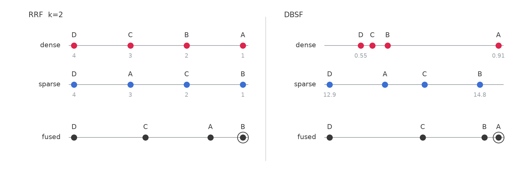
RRF ignores score scale, so a cosine similarity and a BM25 score combine without either dominating. DBSF assumes the size of a score gap means something, so one outlying score can move the result. Which one wins depends on your data, so run both against your labels.
Compare RRF and DBSF on Your Labels
Use your labeled query set to compare RRF and DBSF over the same prefetches. Run RRF at k=2 and equal weights, then run DBSF.
Both queries read the same two candidate lists, so connect once and build the prefetches once. The prefetches must use the models the collection was indexed with.
from qdrant_client import QdrantClient, models
from your_embedding_setup import dense_query, sparse_query

client = QdrantClient(
    url="https://YOUR-CLUSTER.cloud.qdrant.io",
    api_key="<your-api-key>",
)

dense_prefetch = models.Prefetch(query=dense_query, using="dense", limit=200)
sparse_prefetch = models.Prefetch(query=sparse_query, using="bm25", limit=200)
prefetches = [dense_prefetch, sparse_prefetch]
RrfQuery carries both RRF settings, k and the weight pair, shown here at their defaults. It requires Qdrant v1.17 or later and a compatible qdrant-client release.
rrf_response = client.query_points(
    collection_name="products",
    prefetch=prefetches,
    query=models.RrfQuery(rrf=models.Rrf(k=2, weights=[1.0, 1.0])),
    limit=10,
)
The DBSF query differs only in the fusion step.
dbsf_response = client.query_points(
    collection_name="products",
    prefetch=prefetches,
    query=models.FusionQuery(fusion=models.Fusion.DBSF),
    limit=10,
)
On three of these five datasets, DBSF scored higher than default RRF by a margin whose 95% interval excludes zero. SciFact’s 0.0148 gain and ArguAna’s 0.0045 loss both cross zero, so those two datasets are inconclusive.
| Dataset | DBSF | Over Default RRF |
|---|---|---|
| ArguAna | 0.5171 | -0.0045 |
| CodeSearchNet | 0.6716 | +0.0161 |
| SciFact | 0.7323 | +0.0148 |
| DBPedia-entity | 0.4822 | +0.0184 |
| WANDS | 0.7637 | +0.0383 |
DBSF takes no parameters: k and the weight pair are RRF settings, and the public API accepts them only on an RrfQuery. So if DBSF wins on your labels, skip the next two sections and go to the held-out check.
Use Labels to Choose a k Range
Qdrant scores a document at position pos in one prefetch as 1 / ((pos + 1) / weight + k - 1), then sums across prefetches. With equal weights that reduces to 1 / (pos + k), and k alone decides how steeply the head of a list outranks its tail.
Rank 1 outweighs rank 10 by 2.80 times at k=5 and 1.45 times at k=20, so most of the movement sits below k=20. A sweep in even steps of five would spend most of its runs past the point where the curve stops moving.
Sweep k over 1, 2, 5, 20, and 61, changing only k in models.Rrf and keeping equal weights. Lower values favor a document one prefetch ranks highly, and higher values give more credit to documents both prefetches retrieve.
The table gives nDCG@10 at equal weights across five values of k, with k=2 as default RRF. A star marks the best k in each row.
| Dataset | Queries | Relevant per Query | k=1 | k=2 | k=5 | k=20 | k=61 |
|---|---|---|---|---|---|---|---|
| ArguAna | 1,401 | 1.0 | 0.5171 | 0.5216 | 0.5304* | 0.5269 | 0.5207 |
| CodeSearchNet | 1,000 | 1.0 | 0.6501 | 0.6555 | 0.6580* | 0.6511 | 0.6258 |
| SciFact | 300 | 1.1 | 0.7117 | 0.7175* | 0.7154 | 0.7122 | 0.7067 |
| DBPedia-entity | 400 | 38.2 | 0.4625 | 0.4638 | 0.4641 | 0.4682* | 0.4606 |
| WANDS | 480 | 358.9 | 0.7232 | 0.7254 | 0.7336 | 0.7571 | 0.7614* |
On WANDS, k=2 and k=61 chose a different top result for 42% of queries, while nDCG@10 rose by 0.0360. A small aggregate gain can still change what a user sees first.
These five datasets suggest a direction: with about one relevant document per query, the best k was 2 or 5; with tens or hundreds, it was 20 or 61. Count relevant documents per query in your labeled query set, then try that part of the range first.
If you are porting an RRF configuration from another system, remember that Qdrant uses zero-based positions. To reproduce the 1 / (rank + 60) convention from Cormack et al. with one-based ranks, use k=61.
Tune Weights Last
A weight pair gives one multiplier to each prefetch, in the order the prefetches appear in the query. The pair is absolute, so (1, 2) and (2, 4) are two different settings: the formula divides the position by the weight, so scaling both weights changes every score. On WANDS at k=5, (1, 2) scores 0.7390 and (2, 4) scores 0.7508.
Settle k first, since a pair is only valid for the k you tested it with. On WANDS, (2, 4) beats equal weights at k=5. At k=61, that dataset’s best value, equal weights win: 0.7614 against 0.7567.
Then sweep a few pairs and let your labels pick the winner. A prefetch’s own score does not say which way to lean. Weights act on positions inside each list, so the pair is decided by which prefetch ranks relevant documents highly on the queries the other one misses.
On DBPedia-entity, dense retrieval scores 0.4677 against sparse retrieval’s 0.3857, yet the winning pair (1, 3) gives sparse three times the dense weight and gains 0.0060. CodeSearchNet leans the other way and gains 0.0096 at (2, 1). Both intervals exclude zero.
Equal weights are a real outcome. Six pairs ran at each dataset’s best k, and (1, 1) won outright on two of the five. ArguAna’s best pair gained 0.0029, with an interval that crosses zero.
A weight of 0.0 keeps every document from that prefetch and scores each one 0.0. The documents stay at the bottom of the fused list instead of disappearing.
Confirm the Selected Configuration on Held-Out Queries
A configuration can score best on the queries used to select it and still fail on held-out queries. Run both checks from the pre-tuning article: a bootstrap interval on per-query gain, and a split between selection and held-out queries. Ship a configuration when its interval excludes zero and its selected gain holds on the held-out half.
On SciFact’s 300 queries, nothing we tried had a 95% interval that excluded zero, including DBSF’s 0.0148 gain. Across 200 random splits, a selected fusion configuration kept 67% to 95% of its gain on held-out queries. Keeping the default is a real answer, and it was the right one on one of our five datasets.
Tune in This Order
Each step is cheap enough to run in a single session.
- Confirm fusion beats either prefetch alone.
- Pick RRF or DBSF on your labels.
- Set
kfrom the number of relevant documents per query. - Sweep a few weight pairs at that
k. - Validate the winner on held-out queries before shipping.
Next, if a downstream model could improve the ranking of your retrieved candidates, test whether a reranker is worth its cost.
 Ready to try Qdrant?