
It’s been over a year since we published the original article on how to build a hybrid search system with Qdrant. The idea was straightforward: combine the results from different search methods to improve retrieval quality. Back in 2023, you still needed to use an additional service to bring lexical search capabilities and combine all the intermediate results. Things have changed since then. Once we introduced support for sparse vectors, the additional search service became obsolete, but you were still required to combine the results from different methods on your end.
Qdrant 1.10 introduces a new Query API that lets you build a search system by combining different search methods to improve retrieval quality. Everything is now done on the server side, and you can focus on building the best search experience for your users. In this article, we will show you how to utilize the new Query API to build a hybrid search system.
Introducing the new Query API
At Qdrant, we believe that vector search capabilities go well beyond a simple search for nearest neighbors.
That’s why we provided separate methods for different search use cases, such as search, recommend, or discover.
With the latest release, we are happy to introduce the new Query API, which combines all of these methods into a single
endpoint and also supports creating nested multistage queries that can be used to build complex search pipelines.
If you are an existing Qdrant user, you probably have a running search mechanism that you want to improve, whether sparse or dense. Doing any changes should be preceded by a proper evaluation of its effectiveness.
How effective is your search system?
None of the experiments makes sense if you don’t measure the quality. How else would you compare which method works
better for your use case? The most common way of doing that is by using the standard metrics, such as precision@k,
MRR, or NDCG. There are existing libraries, such as ranx, that can help you with
that. We need to have the ground truth dataset to calculate any of these, but curating it is a separate task.
from ranx import Qrels, Run, evaluate

# Qrels, or query relevance judgments, keep the ground truth data
qrels_dict = { "q_1": { "d_12": 5, "d_25": 3 },
               "q_2": { "d_11": 6, "d_22": 1 } }

# Runs are built from the search results
run_dict = { "q_1": { "d_12": 0.9, "d_23": 0.8, "d_25": 0.7,
                      "d_36": 0.6, "d_32": 0.5, "d_35": 0.4  },
             "q_2": { "d_12": 0.9, "d_11": 0.8, "d_25": 0.7,
                      "d_36": 0.6, "d_22": 0.5, "d_35": 0.4  } }

# We need to create both objects, and then we can evaluate the run against the qrels
qrels = Qrels(qrels_dict)
run = Run(run_dict)

# Calculating the NDCG@5 metric is as simple as that
evaluate(qrels, run, "ndcg@5")
Available embedding options with Query API
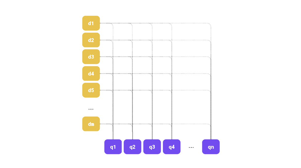
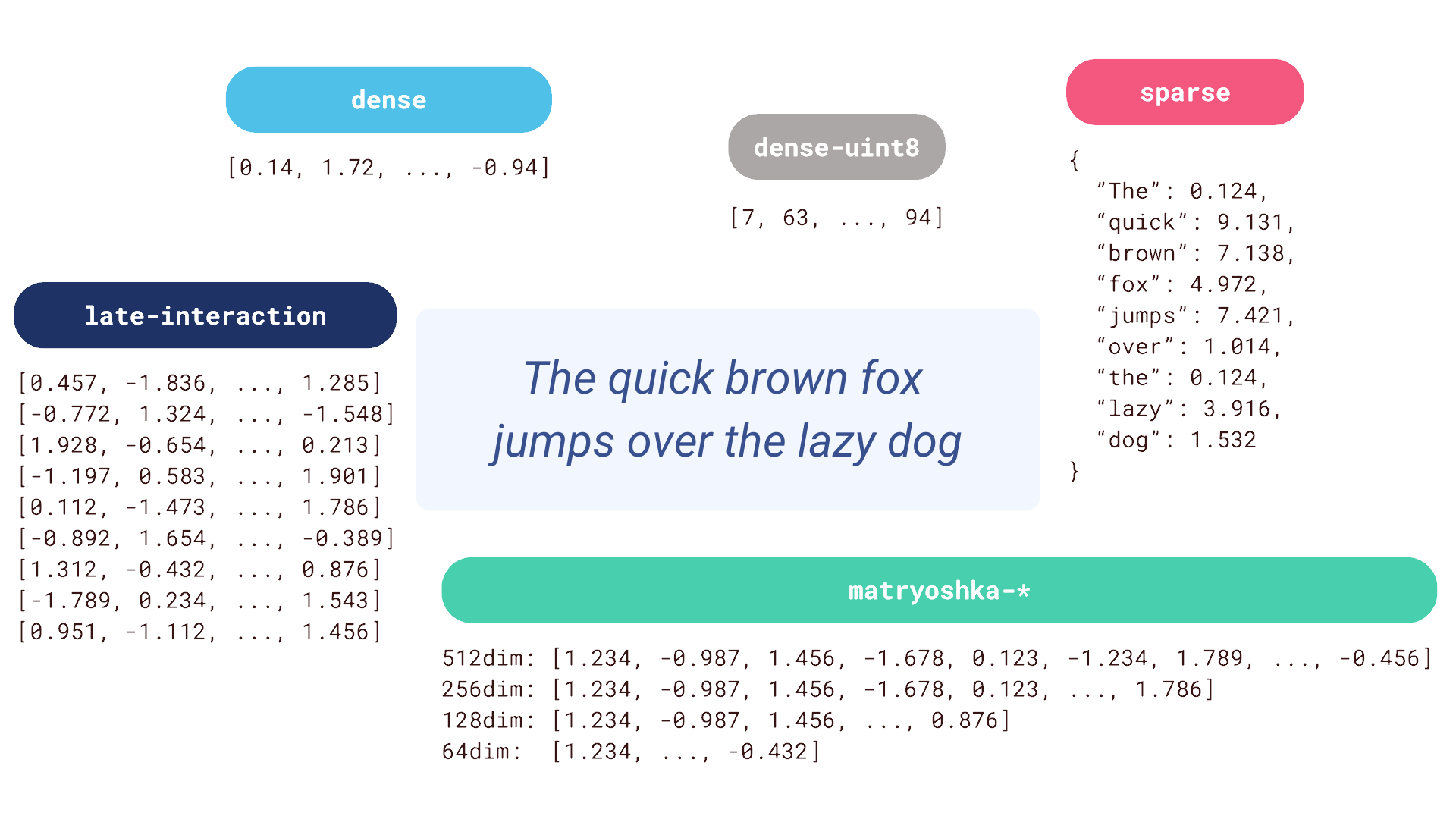
Support for multiple vectors per point is nothing new in Qdrant, but introducing the Query API makes it even more powerful. The 1.10 release supports the multivectors, allowing you to treat embedding lists as a single entity. There are many possible ways of utilizing this feature, and the most prominent one is the support for late interaction models, such as ColBERT. Instead of having a single embedding for each document or query, this family of models creates a separate one for each token of text. In the search process, the final score is calculated based on the interaction between the tokens of the query and the document. Contrary to cross-encoders, document embedding might be precomputed and stored in the database, which makes the search process much faster. If you are curious about the details, please check out the article about ColBERT, written by our friends from Jina AI.
Besides multivectors, you can use regular dense and sparse vectors, and experiment with smaller data types to reduce memory use. Named vectors can help you store different dimensionalities of the embeddings, which is useful if you use multiple models to represent your data, or want to utilize the Matryoshka embeddings.
There is no single way of building a hybrid search. The process of designing it is an exploratory exercise, where you need to test various setups and measure their effectiveness. Building a proper search experience is a complex task, and it’s better to keep it data-driven, not just rely on the intuition.
Fusion vs reranking
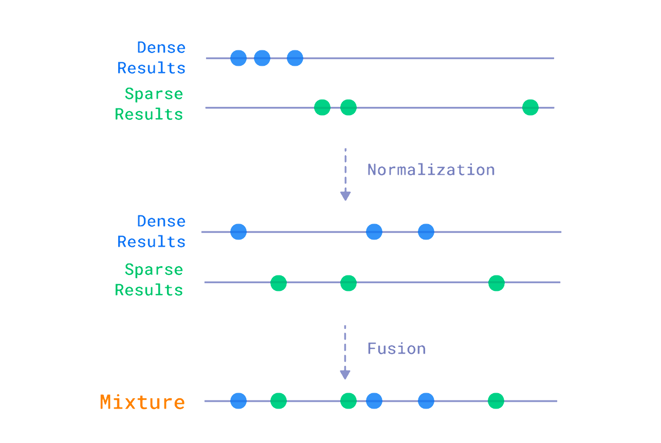
We can, distinguish two main approaches to building a hybrid search system: fusion and reranking. The former is about combining the results from different search methods, based solely on the scores returned by each method. That usually involves some normalization, as the scores returned by different methods might be in different ranges. After that, there is a formula that takes the relevancy measures and calculates the final score that we use later on to reorder the documents. Qdrant has built-in support for the Reciprocal Rank Fusion method, which is the de facto standard in the field.
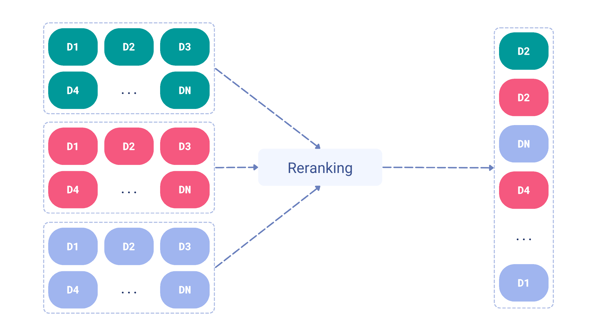
Reranking, on the other hand, is about taking the results from different search methods and reordering them based on some additional processing using the content of the documents, not just the scores. This processing may rely on an additional neural model, such as a cross-encoder which would be inefficient enough to be used on the whole dataset. These methods are practically applicable only when used on a smaller subset of candidates returned by the faster search methods. Late interaction models, such as ColBERT, are way more efficient in this case, as they can be used to rerank the candidates without the need to access all the documents in the collection.
Why not a linear combination?
It’s often proposed to use full-text and vector search scores to form a linear combination formula to rerank the results. So it goes like this:
final_score = 0.7 * vector_score + 0.3 * full_text_score
However, we didn’t even consider such a setup. Why? Those scores don’t make the problem linearly separable. We used the BM25 score along with cosine vector similarity to use both of them as points coordinates in 2-dimensional space. The chart shows how those points are distributed:
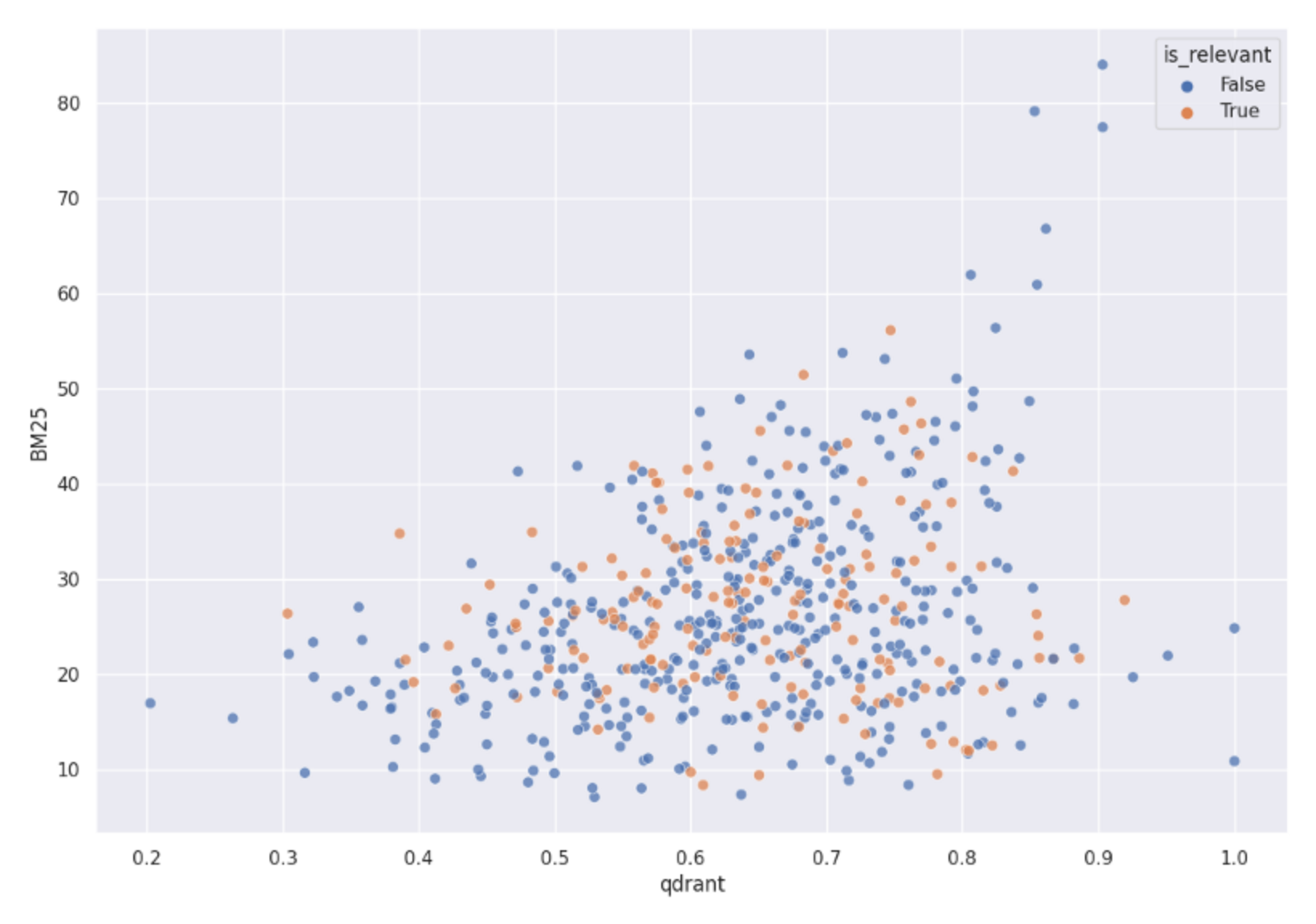
A distribution of both Qdrant and BM25 scores mapped into 2D space. It clearly shows relevant and non-relevant objects are not linearly separable in that space, so using a linear combination of both scores won’t give us a proper hybrid search.
Both relevant and non-relevant items are mixed. None of the linear formulas would be able to distinguish between them. Thus, that’s not the way to solve it.
Building a hybrid search system in Qdrant
Ultimately, any search mechanism might also be a reranking mechanism. You can prefetch results with sparse vectors and then rerank them with the dense ones, or the other way around. Or, if you have Matryoshka embeddings, you can start with oversampling the candidates with the dense vectors of the lowest dimensionality and then gradually reduce the number of candidates by reranking them with the higher-dimensional embeddings. Nothing stops you from combining both fusion and reranking.
Let’s go a step further and build a hybrid search mechanism that combines the results from the Matryoshka embeddings, dense vectors, and sparse vectors and then reranks them with the late interaction model. In the meantime, we will introduce additional reranking and fusion steps.
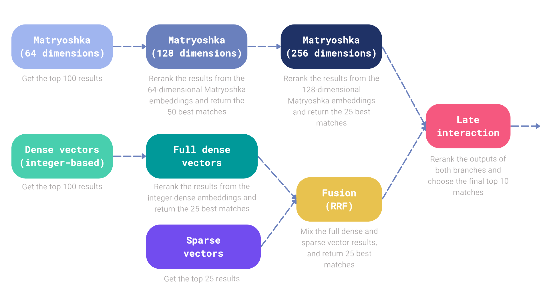
Our search pipeline consists of two branches, each of them responsible for retrieving a subset of documents that we eventually want to rerank with the late interaction model. Let’s connect to Qdrant first and then build the search pipeline.
from qdrant_client import QdrantClient, models

client = QdrantClient("http://localhost:6333")
All the steps utilizing Matryoshka embeddings might be specified in the Query API as a nested structure:
# The first branch of our search pipeline retrieves 25 documents
# using the Matryoshka embeddings with multistep retrieval.
matryoshka_prefetch = models.Prefetch(
    prefetch=[
        models.Prefetch(
            prefetch=[
                # The first prefetch operation retrieves 100 documents
                # using the Matryoshka embeddings with the lowest
                # dimensionality of 64.
                models.Prefetch(
                    query=[0.456, -0.789, ..., 0.239],
                    using="matryoshka-64dim",
                    limit=100,
                ),
            ],
            # Then, the retrieved documents are re-ranked using the
            # Matryoshka embeddings with the dimensionality of 128.
            query=[0.456, -0.789, ..., -0.789],
            using="matryoshka-128dim",
            limit=50,
        )
    ],
    # Finally, the results are re-ranked using the Matryoshka
    # embeddings with the dimensionality of 256.
    query=[0.456, -0.789, ..., 0.123],
    using="matryoshka-256dim",
    limit=25,
)
Similarly, we can build the second branch of our search pipeline, which retrieves the documents using the dense and sparse vectors and performs the fusion of them using the Reciprocal Rank Fusion method:
# The second branch of our search pipeline also retrieves 25 documents,
# but uses the dense and sparse vectors, with their results combined
# using the Reciprocal Rank Fusion.
sparse_dense_rrf_prefetch = models.Prefetch(
    prefetch=[
        models.Prefetch(
            prefetch=[
                # The first prefetch operation retrieves 100 documents
                # using dense vectors using integer data type. Retrieval
                # is faster, but quality is lower.
                models.Prefetch(
                    query=[7, 63, ..., 92],
                    using="dense-uint8",
                    limit=100,
                )
            ],
            # Integer-based embeddings are then re-ranked using the
            # float-based embeddings. Here we just want to retrieve
            # 25 documents.
            query=[-1.234, 0.762, ..., 1.532],
            using="dense",
            limit=25,
        ),
        # Here we just add another 25 documents using the sparse
        # vectors only.
        models.Prefetch(
            query=models.SparseVector(
                indices=[125, 9325, 58214],
                values=[-0.164, 0.229, 0.731],
            ),
            using="sparse",
            limit=25,
        ),
    ],
    # RRF is activated below, so there is no need to specify the
    # query vector here, as fusion is done on the scores of the
    # retrieved documents.
    query=models.FusionQuery(
        fusion=models.Fusion.RRF,
    ),
)
The second branch could have already been called hybrid, as it combines the results from the dense and sparse vectors with fusion. However, nothing stops us from building even more complex search pipelines.
Here is how the target call to the Query API would look like in Python:
client.query_points(
    "my-collection",
    prefetch=[
        matryoshka_prefetch,
        sparse_dense_rrf_prefetch,
    ],
    # Finally rerank the results with the late interaction model. It only
    # considers the documents retrieved by all the prefetch operations above.
    # Return 10 final results.
    query=[
        [1.928, -0.654, ..., 0.213],
        [-1.197, 0.583, ..., 1.901],
        ...,
        [0.112, -1.473, ..., 1.786],
    ],
    using="late-interaction",
    with_payload=False,
    limit=10,
)
The options are endless, the new Query API gives you the flexibility to experiment with different setups. You rarely need to build such a complex search pipeline, but it’s good to know that you can do that if needed.
Lessons learned: multi-vector representations
Many of you have already started building hybrid search systems and reached out to us with questions and feedback. We’ve seen many different approaches, however one recurring idea was to utilize multi-vector representations with ColBERT-style models as a reranking step, after retrieving candidates with single-vector dense and/or sparse methods. This reflects the latest trends in the field, as single-vector methods are still the most efficient, but multivectors capture the nuances of the text better.
Assuming you never use late interaction models for retrieval alone, but only for reranking, this setup comes with a hidden cost. By default, each configured dense vector of the collection will have a corresponding HNSW graph created. Even, if it is a multi-vector.
from qdrant_client import QdrantClient, models

client = QdrantClient(...)
client.create_collection(
    collection_name="my-collection",
    vectors_config={
        "dense": models.VectorParams(...),
        "late-interaction": models.VectorParams(
            size=128,
            distance=models.Distance.COSINE,
            multivector_config=models.MultiVectorConfig(
                comparator=models.MultiVectorComparator.MAX_SIM
            ),
        )
    },
    sparse_vectors_config={
        "sparse": models.SparseVectorParams(...)
    },
)
Reranking will never use the created graph, as all the candidates are already retrieved. Multi-vector ranking will only be applied to the candidates retrieved by the previous steps, so no search operation is needed. HNSW becomes redundant while still the indexing process has to be performed, and in that case, it will be quite heavy. ColBERT-like models create hundreds of embeddings for each document, so the overhead is significant. To avoid it, you can disable the HNSW graph creation for this kind of model:
client.create_collection(
    collection_name="my-collection",
    vectors_config={
        "dense": models.VectorParams(...),
        "late-interaction": models.VectorParams(
            size=128,
            distance=models.Distance.COSINE,
            multivector_config=models.MultiVectorConfig(
                comparator=models.MultiVectorComparator.MAX_SIM
            ),
            hnsw_config=models.HnswConfigDiff(
                m=0,  # Disable HNSW graph creation
            ),
        )
    },
    sparse_vectors_config={
        "sparse": models.SparseVectorParams(...)
    },
)
You won’t notice any difference in the search performance, but the use of resources will be significantly lower when you upload the embeddings to the collection.
Some anecdotal observations
Neither of the algorithms performs best in all cases. In some cases, keyword-based search will be the winner and vice-versa. The following table shows some interesting examples we could find in the WANDS dataset during experimentation:
| Query | BM25 Search | Vector Search |
|---|---|---|
| cybersport desk | desk ❌ | gaming desk ✅ |
| plates for icecream | "eat" plates on wood wall décor ❌ | alicyn 8.5 '' melamine dessert plate ✅ |
| kitchen table with a thick board | craft kitchen acacia wood cutting board ❌ | industrial solid wood dining table ✅ |
| wooden bedside table | 30 '' bedside table lamp ❌ | portable bedside end table ✅ |
Also examples where keyword-based search did better:
| Query | BM25 Search | Vector Search |
|---|---|---|
| computer chair | vibrant computer task chair ✅ | office chair ❌ |
| 64.2 inch console table | cervantez 64.2 '' console table ✅ | 69.5 '' console table ❌ |
Try the New Query API in Qdrant 1.10
The new Query API introduced in Qdrant 1.10 is a game-changer for building hybrid search systems. You don’t need any additional services to combine the results from different search methods, and you can even create more complex pipelines and serve them directly from Qdrant.
Our webinar on Building the Ultimate Hybrid Search takes you through the process of building a hybrid search system with Qdrant Query API. If you missed it, you can watch the recording, or check the notebooks.
If you have any questions or need help with building your hybrid search system, don’t hesitate to reach out to us on Discord.