
Why Hyperbolic Embeddings Matter for Hierarchical Data
Matin Mahmood and John Kupchanko
·September 08, 2026

We choose embedding models, dimensions, and indexes. The geometry usually comes with the package. But why use a flat space, and what else could we choose?
What Is a Manifold, and Where Do Our Vectors Live?
A manifold is the space our embeddings live in. For embeddings, we care about the geometry we give that space. It determines how we measure distance, what the shortest path looks like, and how much room there is as we move outward.
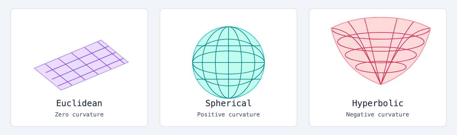
Euclidean, spherical, and hyperbolic spaces. The hyperbolic space is shown using the Lorentz model.
The embedding is still a vector. The geometry determines how we measure distance between vectors.
| Space | Geometry | A natural example |
|---|---|---|
| Euclidean | Flat | Continuous positions and attributes |
| Spherical | Positively curved | Angular or periodic data |
| Hyperbolic | Negatively curved | Branching hierarchies |
Many familiar embedding models normalize their vectors onto a sphere and use cosine similarity. Hyperbolic embeddings use a different geometry, one that is particularly well suited to branching relationships.
Hierarchical Data Meets Hyperbolic Embeddings
Imagine a product catalog. Footwear splits into boots, trainers, and sandals. Boots split into ankle boots, hiking boots, and work boots. Each type contains products, and each product can have several variants.
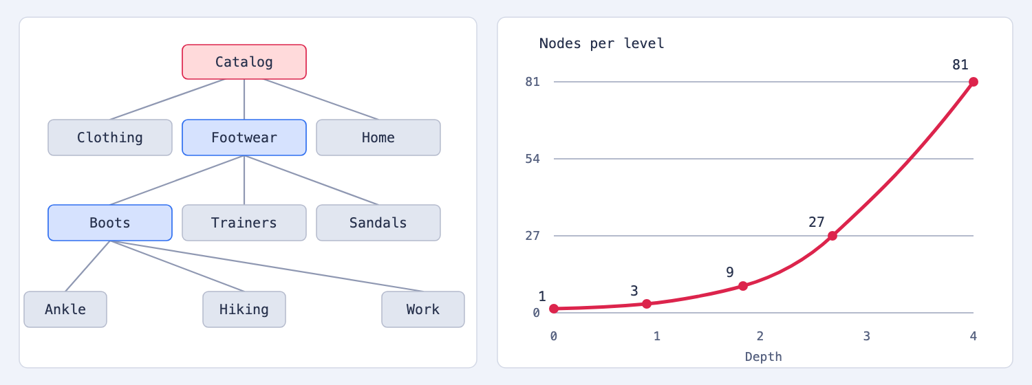
A catalog with three children per node grows as $3^\ell$ at depth $\ell$.
A tree multiplies. A flat disk only squares.
In $d$-dimensional Euclidean space, the volume within radius $r$ grows polynomially:
$$ V_E(r) \propto r^d. $$
In two-dimensional hyperbolic space with curvature $-1$, the area is
$$ A_H(r)=2\pi(\cosh r-1), $$
which grows exponentially for large $r$.
That is a much closer match to the growth of a branching tree. As a hierarchy gets deeper, hyperbolic space keeps creating room for its descendants. In a flat space, branches increasingly crowd together.
The same branching structure appears in biological taxonomies, document hierarchies, and part and whole relationships. Hyperbolic embeddings give these hierarchies room to grow.
Superpowers of Hyperbolic Embeddings
Matching the geometry to the data can make an embedding more compact and give its coordinates more meaning. Two useful examples are dimensional efficiency and radius as a measure of specificity.
Dimensional Efficiency
When the geometry matches the data, you can often represent the same structure with fewer dimensions.
WordNet gives a concrete example. Its noun hierarchy contains relationships such as poodle → dog → animal. We can compare how well Euclidean and hyperbolic embeddings reconstruct those relationships at different dimensions. [1]
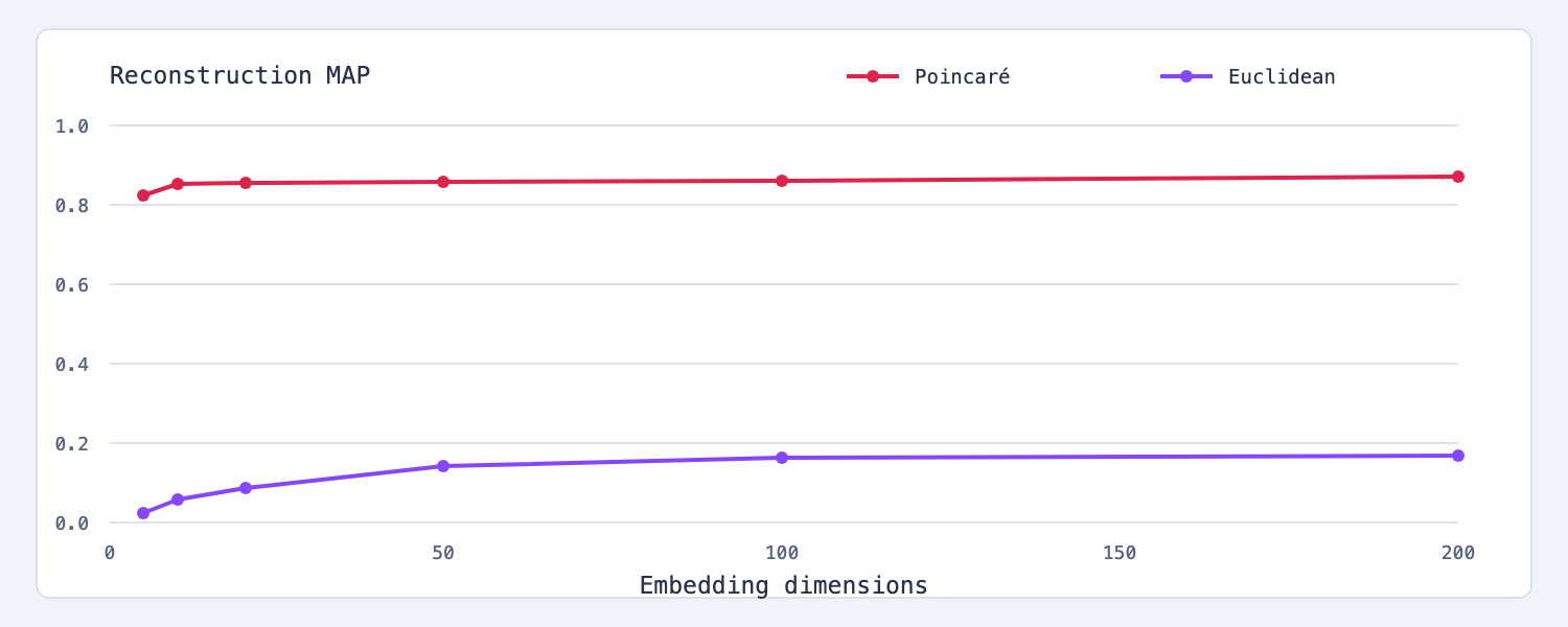
WordNet reconstruction, measured by mean average precision (higher is better). Results from Table 1. [1]
Five-dimensional Poincaré embeddings achieved 0.823, compared with 0.168 for 200-dimensional Euclidean embeddings. That is 40 times fewer coordinates and better reconstruction on this task.
Fewer coordinates mean fewer values to store and move through a retrieval system. Before reaching for a larger vector, it is worth asking whether a different geometry would fit the data better.
Radius Can Encode Specificity
One of the nicest properties of a hierarchy-aware hyperbolic embedding is that radius can start to mean something.
Closer to the center, you can place broad concepts. Farther out, you can place more specific descendants. Direction separates branches; radius helps organize depth.
For a catalog, “footwear” covers many possible items. “Boots” narrows that set. “Red leather ankle boots” narrows it further. A representation that captures this structure has room for both semantic similarity and different levels of detail.
Hyper3-CLIP, a hyperbolic image and text embedding model from hyper³labs, brings this idea to visual retrieval. [7] It is trained to capture general-to-specific relationships alongside similarity. This gives radius a role in organizing broad descriptions and specific visual content. [2] It follows earlier work on hyperbolic image and text representations. [3]
Hyper3-CLIP appears here to illustrate what radius can carry. It is not the model benchmarked later: the tests below use a small embedding we trained ourselves on a single taxonomy.
Consider the black Chelsea boot in the next figure. A traversal toward the origin illustrates a move from the specific product to broader concepts: black Chelsea boots, Chelsea boots, boots, and footwear.
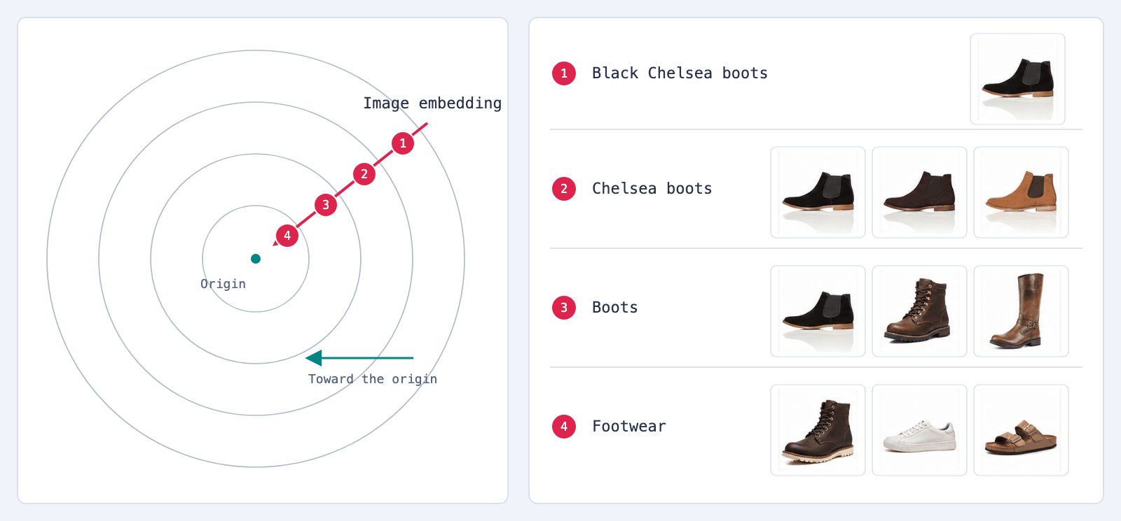
Conceptual traversal inspired by a catalog product from Amazon Berkeley Objects. Product imagery is AI-illustrated; descriptions and positions are illustrative, not model retrieval results. [6]
We can also look at how the model organizes product images. The next figure compares conventional CLIP [8] and Hyper3-CLIP embeddings of the same catalog subset.
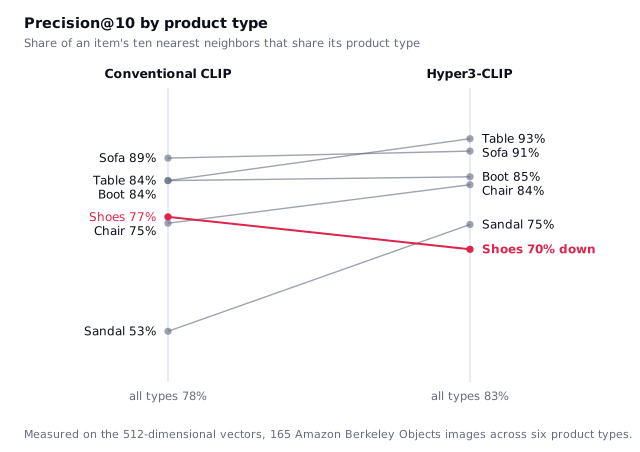
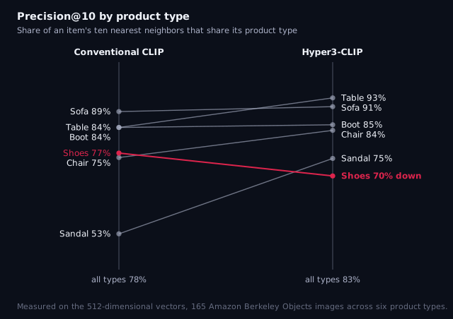
This is a retrieval measurement rather than a picture of a layout. Neighborhoods are taken from the 512-dimensional vectors, not from any projection of them, so nothing here depends on how the points were arranged for display. The gain is not uniform: Sandal improves by 22 points, Shoes gets worse by 7, and the average over all six types moves from 0.778 to 0.834. [9]
Testing Hyperbolic Embeddings
WordNet is useful for showing why hyperbolic embeddings work, but we also wanted to see what happens on something closer to a real application. So we tested the same idea on the Google Product Taxonomy: 5,595 categories, seven levels, and 17,312 relationships. [10]
We trained both embeddings ourselves so that the data, the dimension, and the optimizer are held constant and only the geometry changes. An off-the-shelf model would have varied all of them at once. They are deliberately small: five dimensions is a research setting, not a production recommendation.
We scored them with mean average precision, written MAP from here on. It asks how close each category’s true parents land to the top of its results. Higher is better, and 1.000 MAP would mean every parent came back first.
| Dimensions | Euclidean MAP | Poincaré MAP |
|---|---|---|
| 2 | 0.140 | 0.501 |
| 5 | 0.239 | 0.905 |
| 10 | 0.354 | 0.925 |
| 20 | 0.551 | 0.932 |
| 50 | 0.658 | 0.934 |
At just 5 dimensions, the Poincaré embedding reaches 0.905 MAP. The Euclidean version only reaches 0.658 MAP at 50 dimensions, using ten times as many coordinates.
That is the part that matters. When the data really does branch like a tree, hyperbolic geometry can represent that structure much more efficiently.
There is one limitation. These numbers measure relationships the embedding already saw during training. When we asked it to find each category’s direct parent instead, the score dropped to 0.539 MAP.
So we would not treat this as a universal win. We would treat it as a strong reason to test hyperbolic embeddings when the data itself is hierarchical.
Serving Them with Qdrant
Getting a good embedding was only half the problem. The next question was how to search it.
Hyperbolic distance can be converted into an inner product by adding two extra dimensions. Under brute force search in Faiss, that worked well. Across 82,115 WordNet nouns it found 0.986 of the correct nearest neighbors in its top 10, a measure we write as recall@10.
Then we put the same vectors behind Faiss’s HNSW index. Recall@10 dropped to 0.020, even with ef=1024. That figure is Faiss, not Qdrant.
The conversion was still mathematically correct, but the resulting vectors had norms spread across roughly a 600x range, which is hard on a proximity graph built from inner products. Grouping vectors by norm helped, but recall@10 only reached 0.410. Both figures are from the same Faiss setup.
So instead of forcing the converted vectors into HNSW, we changed the search strategy.
The collection stores the Poincaré coordinates as an ordinary Euclidean vector, and keeps each point’s squared norm in its payload:
client.create_collection(
    "taxonomy_geometry",
    vectors_config={
        "hyperbolic": models.VectorParams(size=5, distance=models.Distance.EUCLID),
    },
)

client.create_payload_index(
    "taxonomy_geometry", "sq_norm",
    field_schema=models.PayloadSchemaType.FLOAT,
)
Without that payload index the rescore turns into a full scan.
Qdrant first uses Euclidean HNSW to pull a candidate set from the original Poincaré coordinates. Then a Formula Query rescores those candidates with the real hyperbolic distance in the same request. [5]
Euclidean is the prefetch metric here because away from the edge of the ball it tracks hyperbolic distance closely enough to gather candidates. Cosine is the obvious alternative, and which one wins depends on how wide the prefetch is. At a prefetch of 50 cosine is ahead, 0.505 against 0.472. At the prefetch of 1,000 this article recommends it is behind, 0.876 against 0.920, and it does not catch up: cosine’s recall saturates near 0.875 at every width we tried. Direction alone finds the right neighborhood but cannot separate depths inside it, which is what the rescore is for.
The geodesic, meaning the shortest path between two points in the curved space, is the true hyperbolic distance. Computing it needs acosh, the inverse hyperbolic cosine, and Formula Query did not have that operator when we ran these tests. An acosh expression was merged into Qdrant in August 2026 [4], but it was not part of a stable release as of v1.19.1. Formula Query does have ln and sqrt, and since acosh(x) is ln(x + sqrt(x^2 - 1)), the distance is expressible as it stands. The inner term is:
{
  "sum": [1.0, {"div": {
    "left":  {"mult": [2.0, {"pow": {"base": "$score", "exponent": 2.0}}]},
    "right": {"mult": [0.0488, {"sum": [1.0, {"neg": "sq_norm"}]}]}
  }}]
}
$score is the Euclidean distance the prefetch already computed. sq_norm comes from the payload. 0.0488 is one minus the squared norm of the query, which you calculate before sending. The vector here is the stored point for Animals & Pet Supplies, whose squared norm is 0.9512. Call that term x, and the query is:
{
  "prefetch": [{
      "query": [-0.3189, 0.9057, -0.0140, 0.1646, -0.0439],
      "using": "hyperbolic",
      "limit": 1000
    }],
  "query": {"formula": {
    "neg": {"ln": {"sum": [
      x, {"sqrt": {"sum": [{"pow": {"base": x, "exponent": 2.0}}, -1.0]}}
    ]}}
  }},
  "limit": 10
}
We tested this against a live Qdrant collection with all 5,595 taxonomy points. At that size Qdrant serves the collection by exact search rather than building a graph, so these are exact-search numbers. Forcing the graph on changes them by at most 0.002.
| Prefetch | Euclidean Only | With Rescore |
|---|---|---|
| 10 | 0.266 | 0.257 |
| 50 | 0.266 | 0.472 |
| 100 | 0.266 | 0.598 |
| 300 | 0.266 | 0.783 |
| 1000 | 0.266 | 0.920 |
Euclidean prefetch alone finds about a quarter of the correct hyperbolic neighbors. With a prefetch of 1,000 and Formula Query rescoring, recall@10 reaches 0.920. And the whole search stays inside Qdrant in one server side request.
The prefetch size matters. If the right neighbors never make it into the candidate set, rescoring cannot recover them.
There is one more tradeoff. As the embedding gets better, the prefetch usually needs to get wider.
Comparing two embeddings offline, the stronger one at 0.905 MAP recovered 0.498 of the true neighbors from a prefetch of 50, while a weaker one at 0.724 MAP recovered 0.789 of them.
Better hyperbolic embeddings push more points toward the edge of the Poincaré ball, where Euclidean distance becomes a weaker shortcut. So if you improve the embedding, retest the retrieval settings too.
What About a Production 512-Dimensional Model?
Everything above uses a five dimensional embedding we trained on one taxonomy. A fair question is what changes if you reach for a pretrained 512 dimensional hyperbolic model instead, such as Hyper3-CLIP. [2] Mostly the answer is that you need less of this article, not more, and the reason is where in the space those vectors sit.
We measured the hyperbolic radius of the output of two open hyperbolic CLIP models. Every point lands in a thin shell close to the origin:
| Model | Median hyperbolic radius | Spread (max/min) |
|---|---|---|
| HyCoCLIP-ViT-S | 0.627 | 1.04 |
| MERU-ViT-S | 0.872 | 1.10 |
Across six very different image classes the per-class standard deviation was about 0.005 on a mean of 0.63. That is a shell, not a distribution, which suggests the concentration is a property of the model rather than of the images.
Near the origin, hyperbolic space is almost flat, so radius carries almost no information and ordinary metrics recover the true ranking anyway. On 300 real vectors compared all against all, plain cosine over the raw vector reached 0.9997 recall@10 against the exact geodesic.
Every failure described in this article is a crowding effect that appears far from the origin, and the taxonomy embedding we trained sits out there. A pretrained hyperbolic CLIP does not. So the practical test is one measurement: take the median hyperbolic radius of your own corpus. Below roughly 2, treat the space as flat and use an ordinary metric. Above it, the prefetch and rescore route is the one you want.
One property makes these models easier to serve than expected. For a model on the hyperboloid, ranking by the Lorentz inner product is rank identical to ranking by geodesic distance. Across 40 queries the Spearman correlation was 1.000000 every time, so acosh is never needed for ranking. Negate the time coordinate before you store the vector and Distance.DOT returns exact hyperbolic order with no rescoring step at all. This is also why such a model can offer a Lorentz score as its default retrieval mode: on the hyperboloid that score already is the hyperbolic ordering.
Two caveats. These numbers come from HyCoCLIP-ViT-S and MERU-ViT-S rather than hyper3-clip-v1, which is gated, and from exact comparison over a few hundred vectors rather than a full index. Treat the radius test as the finding and the rest as a starting point.
Exploring the Results
To make the difference easier to see, we built a live viewer against the same Qdrant collection.
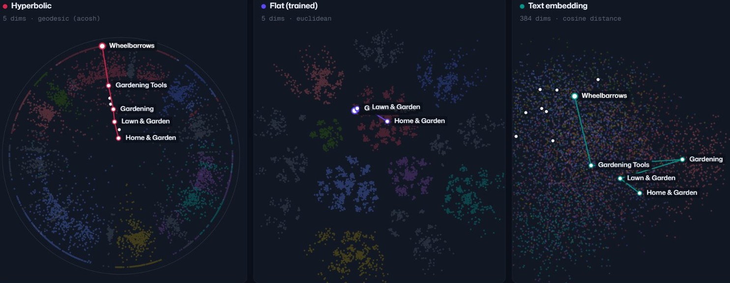
Open the interactive viewer → Pick any of the 5,595 categories and watch all three panels redraw. It runs three searches, one per panel: exact hyperbolic distance, Euclidean distance over the flat trained coordinates, and cosine similarity over a text embedding. The Product Images tab does the same for the CLIP comparison above.
The distances shown in the viewer come directly from Qdrant. Nothing is recalculated in the browser.
We checked the same calculations outside Qdrant, and they matched within 4.7e-07. So the viewer is showing the actual search behavior, not an approximation.
Takeaways
If your data naturally forms a hierarchy, we would test a small hyperbolic embedding before automatically reaching for a much larger Euclidean one. On the product taxonomy, a 5 dimensional Poincaré embedding reached 0.905 MAP. A 50 dimensional Euclidean embedding reached 0.658 MAP.
This pays off when the hierarchy is genuinely deep and parent-to-child structure is what you are searching on. A general catalogue where people type product names is not that case, and a flat model will serve it better.
The harder part is serving it. Converting the vectors and indexing them directly worked under brute force search but collapsed to 0.020 under Faiss’s HNSW, which is why we went looking for another route.
Instead, use HNSW to find candidates and let Qdrant rescore them with the real hyperbolic distance. On this collection, that moved recall@10 from 0.266 to 0.920 with a prefetch of 1,000.
You may also need to widen the prefetch as the embedding improves because Euclidean distance becomes less reliable near the edge of the Poincaré ball.
The main point is simple. If the data is hierarchical, Qdrant gives you a practical way to store the coordinates, use HNSW for candidate retrieval, and apply the real geometry during rescoring without adding a separate search system.
If you want to try this on your own hierarchy, the transform and the two-stage search are packaged in qdrant-hyperbolic-transform. [11] It is a preprocessing layer rather than a change to Qdrant: you convert your vectors, create an ordinary collection with Distance.DOT, and search it normally.
References
- Nickel, M. and Kiela, D. (2017). Poincaré Embeddings for Learning Hierarchical Representations. WordNet reconstruction results: Table 1.
- Mahmood, M. et al. (2026). Hyper3-CLIP: Hierarchy-Conditioned Hyperbolic Vision-Language Training.
- Desai, K. et al. (2023). Hyperbolic Image-Text Representations (MERU).
- Qdrant. Add
acoshexpression to Formula Query. - Qdrant. Hybrid Queries and Formula Query.
- Amazon Berkeley Objects. Product image, item
B06XCPVVPS, image71KwV3JHT9L. - hyper³labs. The Geometry Mistake Behind Modern Embedding Models.
- Radford, A. et al. (2021). Learning Transferable Visual Models From Natural Language Supervision (CLIP).
- Amazon Berkeley Objects. Dataset and documentation.
- Google. Google Product Taxonomy.
- Kupchanko, J. qdrant-hyperbolic-transform. Reference implementation of the transform and the prefetch-and-rescore search.