
Memory Tiers in Qdrant: What to Use and When
A growing vector collection eventually outgrows the RAM it started with: Qdrant handles that by letting you assign dense vectors, the HNSW graph, quantized vectors, payloads, and payload indexes each to whichever memory tier that structure supports, instead of forcing one RAM-versus-disk trade-off onto the whole collection.
This article will give you practical guidance over which combination of tiers and quantization to reach for at each stage of a collection’s growth, and the reasons behind the choice.
How Qdrant’s Memory Tiers Work
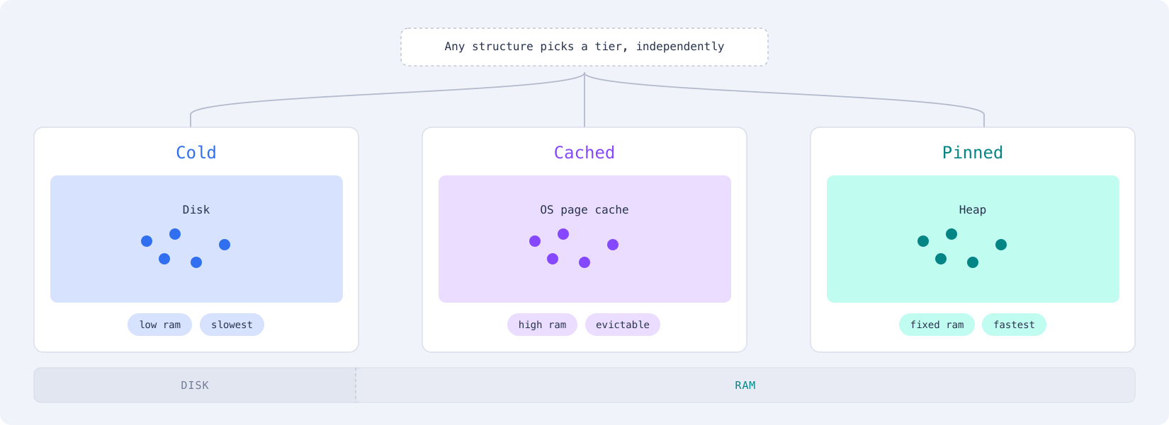
RAM is fast and expensive, disk is slow and cheap, and a growing collection outgrows its RAM budget long before it outgrows its disk budget. Qdrant gives you three tiers to manage that trade-off:
- Pinned. Lives on the heap and never gets evicted, so access is always fast.
- Cached. Memory-mapped and pre-warmed into the OS page cache at startup, so it starts fast too, but the OS can push it out under memory pressure.
- Cold. Also memory-mapped, without the pre-warming, so the first read of any page comes from disk.
Not every structure supports every tier: dense vectors and payloads can’t be pinned, and sparse vector structures follow their own rules. For the full breakdown, see the memory tiers documentation.
Quantization is one of the main tools that makes the cold and pinned tiers practical at real scale. Compressing vectors to int8 or lower shrinks them enough to fit a small, fixed amount of RAM. A search can then score most candidates against that compressed copy instead of paging in the full-precision ones. Rescoring is on by default only for binary quantization and low-precision TurboQuant.
Combining Tiers and Quantization
Tiers and quantization combine into a handful of configurations that cover most collections, from a small one that fits entirely in RAM to one too large for RAM at any budget:
- Full Cached, No Quantization. Dense vectors and the HNSW graph both cached. The simplest option, and a good default as long as the whole working set fits comfortably in RAM.
- Full Cached, With Quantization. The same, plus a compressed copy of the vectors also cached, overriding Qdrant’s default of pinning that copy instead. This keeps two copies of the vector data warm at once, so it only makes sense with RAM to spare for both.
- Full Cold, No Quantization. Dense vectors and the graph both memory-mapped without pre-warming. Minimizes RAM use, but every first touch on a page comes from disk.
- Full Cold, With Quantization. The cold tier, plus a compressed copy that’s also left cold, matching Qdrant’s own default for that combination. Lower disk-read cost than the unquantized cold tier, since most candidates score against the small compressed copy instead.
- Pinned Quantized Vectors. Dense vectors kept cold, but the compressed copy explicitly pinned in RAM. This is the configuration Qdrant’s optimization docs recommend for high-speed search with a low memory footprint, and the one to reach for once RAM headroom becomes the binding constraint.
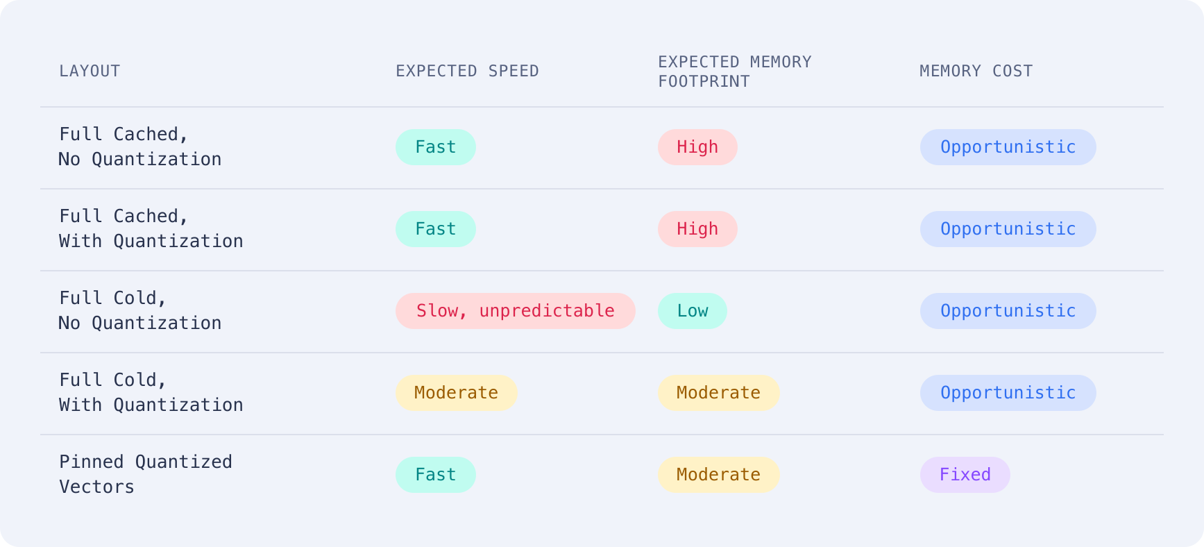
Four of these five configurations leave their memory cost up to the OS: how much of that expected footprint actually stays resident depends on what else is competing for RAM. Only pinning turns that footprint into a fixed reservation instead.
Pin Quantized Vectors for Predictability
Pin the compressed copy once a collection is large enough that RAM becomes the binding constraint, not just raw speed. That fixed reservation is what keeps pinning safe as a collection keeps growing, well past the point where the other configurations start running out of memory headroom.
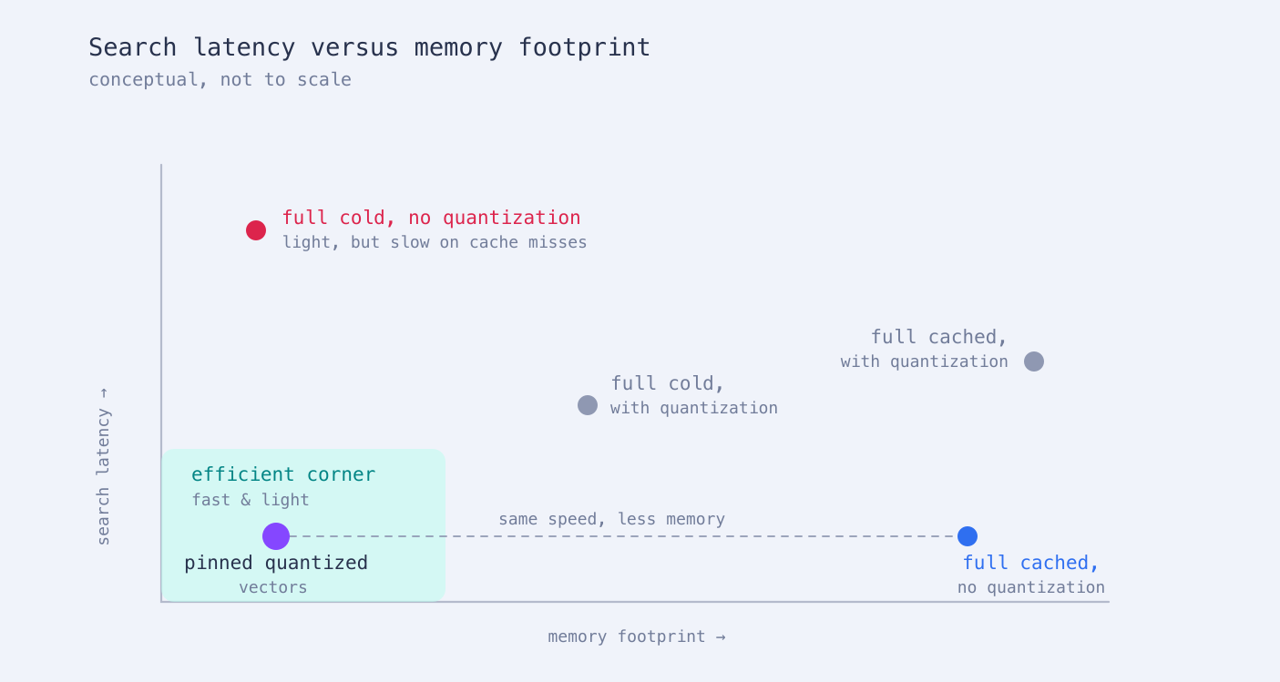
Pinning tends to land in that efficient corner: it matches the fastest configuration’s search speed while using a fraction of its memory footprint. The configurations that leave their footprint up to the OS spike toward the cluster’s memory ceiling as a collection grows, while the pinned one’s footprint barely moves.
On a collection small enough to fit entirely in the cached tier with room to spare, skip pinning: it adds configuration for no speed advantage, since caching the full-precision vectors matches pinning on latency as long as everything actually fits.
Use The Cold Tier With Quantization
If disk footprint matters more than just raw speed, consider adding quantization before fully committing to the cold tier. Every first touch on a cold, unquantized structure comes from disk, and a single HNSW traversal touches enough pages that a rare query can stretch far past its typical latency.
Giving the search a small compressed copy to score against, instead of paging full-precision vectors in from a cold file, removes most of the tail-latency risk even before anything gets pinned.
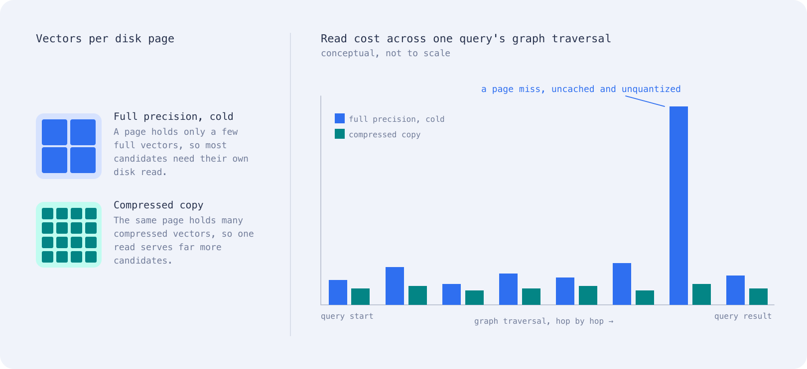
A disk page holds only a handful of full-precision vectors, so most candidates a traversal touches need their own read. A compressed copy packs many more vectors onto the same page, so one read serves far more of the candidates a query needs.
Most queries against an unquantized cold tier still come back fine: the risk is in the tail, where a rare hop lands on a page that isn’t already cached and pays for that read in full, a condition the quantized configurations don’t reproduce.
When To Cache Everything
Don’t cache a compressed copy alongside full-precision vectors unless RAM has room for both. It doubles the resident working set instead of shrinking it, since Qdrant’s default is to pin that compressed copy rather than cache it.
Caching the full-precision vectors alone is fast and simple as long as RAM has room for it. The risk shows up once the working set stops fitting: a configuration that performed close to the fastest option at a smaller scale can fall to nearly the worst as its resident data approaches the cluster’s memory budget.
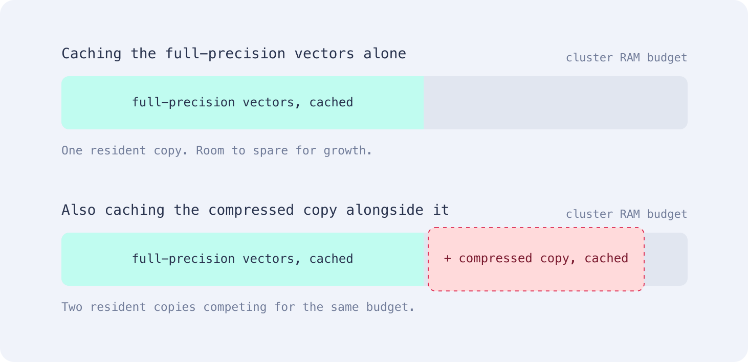
The failure isn’t the tier logic breaking, but the cluster running out of memory to keep that much data warm at once: a sizing problem rather than a caching one, but the cached tier is uniquely exposed to it.
In these cases, the latency can increase by multiple times, and its worst-case queries stretch far past normal, as its working set is very close to the cluster’s memory ceiling.
HNSW Inline Storage and Disk Space
Test HNSW inline storage with quantization at your real vector dimensionality and graph connectivity before relying on it in production. Qdrant’s inline HNSW storage removes a random-access read by copying vector data directly into the graph file: a full-precision copy per point, plus a compressed copy for every edge into it.
That second cost scales with edge count and vector size, not point count, so it can grow far faster than the collection does.
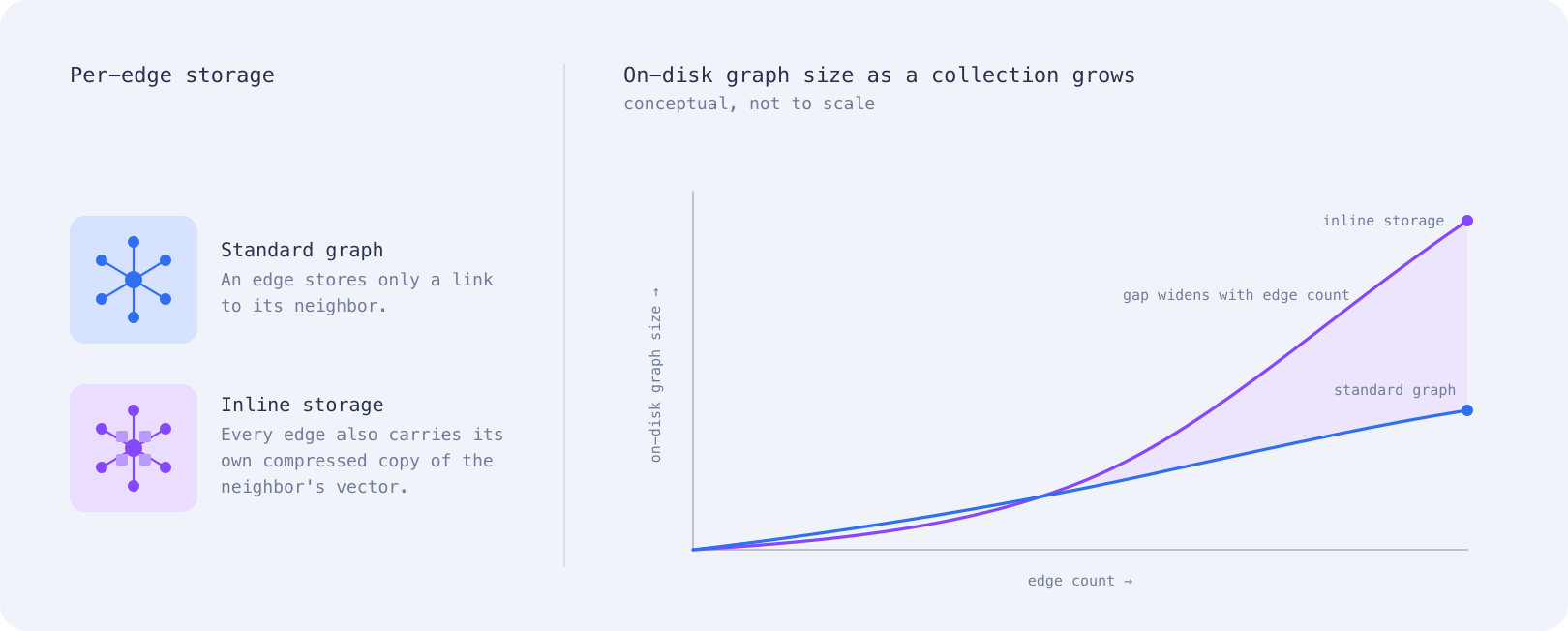
Combining inline storage with quantization can push on-disk graph size to many times larger than the same graph without inline storage. Dense, high-dimensional graphs push the per-edge cost further than sparse, low-dimensional ones, so treat any single multiplier you measure as workload-specific rather than universal. A smaller compressed vector size shrinks it: fewer bytes per edge means less extra disk, though it won’t remove the problem entirely.
Treat RAM as a Limiting Factor
Size each configuration against how much of the cluster’s RAM its working set occupies right now, not how many points the collection holds or the headroom you had at initial setup. A single configuration can look fine, fail, and recover again, purely because the ratio between dataset size and available RAM shifts underneath it.
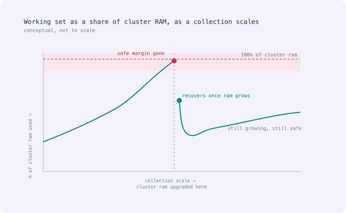
A story built only on point count, where more data always means a worse tail, doesn’t hold up: a caching configuration that looks competitive at a smaller scale can fall apart at a bigger one, once its working set comes near the cluster’s entire memory budget, then look fine again as soon as the cluster’s own RAM budget grows to match.
Takeaways
- Pin the compressed copy once RAM headroom, not raw speed, becomes the binding constraint. Skip it on collections small enough to fit entirely in the cached tier.
- Add quantization before going cold if disk footprint matters more than raw speed; never leave dense vectors cold and unquantized in a latency-sensitive workload.
- Don’t cache a compressed copy alongside full-precision vectors unless the cluster has RAM to spare for both.
- Test HNSW inline storage with quantization at your real vector dimensionality and graph connectivity before trusting it in production.
- Re-check RAM headroom against the working set at every scaling step, not just at initial setup.
Adjacent Work
- Memory tiers documentation: the full set of tier and quantization options per structure.
- Storage documentation: how collections, segments, and storage structures fit together on disk.
- qdrant-labs/memory-tiers-explained: the benchmark code and raw results behind the guidance in this piece.
 Ready to try Qdrant?