
Most retrieval systems run one pipeline on every query, and it is the wrong default in both directions: a single pass under-serves the hard queries, while reranking or rewriting every query wastes compute on the easy ones. Worse, the single pass fails silently. When the relevant document never reaches the top, the system answers anyway from whatever it got, with no sign anything went wrong.
The expensive fixes are well understood, cross-encoders, ColBERT late interaction, query rewriting, and decomposition, so the real question is when to spend them: ideally you catch a weak retrieval cheaply, before paying for any of them, and escalate only the queries that need it. But what tells you, cheaply, that a retrieval is weak? That depends on how your retrieval fails, and we measure it across three corpora.
What “Weak Retrieval” Means
Detecting weak retrieval starts with a measurable definition. Only the top few results are ever used: the top-k chunks fed to the model, or the page shown to a user. Call that the window. Good retrieval puts every piece of evidence the query needs inside it; a retrieval is weak when even one is missing, however good the recall looks deeper down.
Set the window to whatever your system consumes. On a labeled split, where you know which documents each query needed, weak is a binary label you can predict.
Cheap Signals
A signal is a number computed from the result that predicts weak evidence. Two criteria:
- It separates good retrievals from weak ones on labeled data.
- It is cheap enough to run on every query.
“Cheap” rules out the obvious move: asking an LLM “is this enough?” on every query adds a model call to the path you were protecting. The signals here read what the retriever already returned, or at most one extra Qdrant query. No LLM in the hot path.
None of them are new: predicting whether retrieval succeeded is query performance prediction (QPP), and dense_variance is close to its Unnormalized Query Commitment. The contribution is not a new predictor but which known ones earn their cost, and on what kind of corpus.
| Family | Signal | What it reads | Flags weak when |
|---|---|---|---|
| height | max_score | top-1 fused score | low |
| spread | dense_variance | variance of the raw dense cosines | low |
| coverage | evidence_coverage | question entities present in the top-k text | low |
| agreement (dense vs sparse) | retriever_divergence | dense vs sparse top-k overlap | high (they disagree) |
| agreement (across dense models) | dense_agreement | top-k overlap across independent dense models | low (they disagree) |
The intuition is what transfers to a new corpus:
- Height and spread: a confident retriever fans its top scores apart; a lost one bunches them.*
- Coverage: do the entities named in the query appear in the retrieved text.
- Agreement: when two retrievers, or two dense models, return different documents, one is usually lost, most often on jargon and out-of-vocabulary terms.
*Spread only carries information on scores that keep their magnitude. Read it off the raw dense cosines under rank-based RRF, which discards magnitude, or off the fused scores under score-preserving fusion like DBSF.
How the Signals Are Computed
The spread signal is the population variance of the retriever’s scores:
import statistics

def dense_variance(dense_ranking):    # spread of the raw dense cosines
    return statistics.pvariance([score for _, score in dense_ranking])
dense_variance reads the raw dense ranking, one extra Qdrant query that reuses the query vector you already embedded, so no extra model call:
def dense_ranking(query_vector, window_k=10):
    points = client.query_points(
        collection_name="your_collection",
        query=query_vector,
        using="dense",
        limit=window_k,
        with_payload=False,
    ).points
    return [(p.id, p.score) for p in points]
Both agreement signals are top-k set overlap. retriever_divergence compares the dense and sparse rankings; dense_agreement averages overlap across two or more independent dense models. Either way, disagreement means weak retrieval:
from itertools import combinations

def jaccard(a, b):  # set overlap of two top-k id lists
    a, b = set(a), set(b)
    return len(a & b) / len(a | b) if a or b else 1.0

def retriever_divergence(dense_ids, sparse_ids):
    return 1 - jaccard(dense_ids, sparse_ids)  # high when they disagree

def dense_agreement(rankings):  # one top-k id list per model
    scores = [jaccard(a, b) for a, b in combinations(rankings, 2)]
    return sum(scores) / len(scores)  # low when they disagree
The agreement signals are not free: dense_agreement runs the extra dense models, a few embeddings per query. Still far cheaper than an LLM judge.
Which Signals Fire Depends on the Failure Mode
Score each signal by how well it separates good from weak retrievals on a labeled split, using AUC (0.5 chance, 1.0 perfect). We ran all of them on three corpora that fail differently: MuSiQue (multi-hop QA), and the BEIR sets NFCorpus (medical jargon) and SciFact (scientific claims).
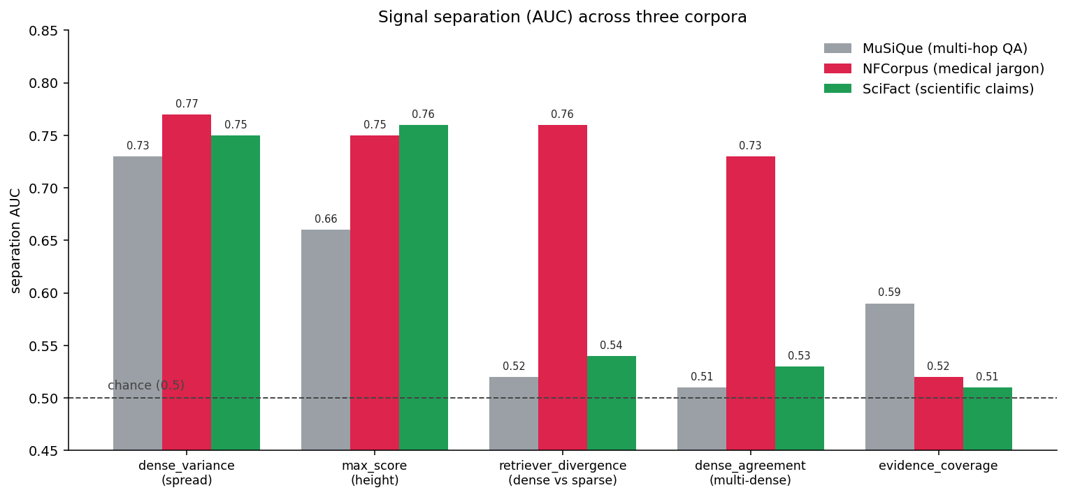
Separation AUC per signal, per corpus. Dense spread transfers across all three; the others help only where the corpus fails their way. Stack: bge-base + miniCOIL fused with RRF, plus mxbai-embed-large and arctic-embed-m for the agreement signals; windows are per corpus, so compare within a column, not across.
No single signal was best on all three, and which ones were worth computing tracked how the corpus failed:
- Vocabulary mismatch (NFCorpus): on this corpus, jargon and out-of-vocabulary terms seem to make dense and sparse, and independent dense models, disagree on weak queries. The agreement signals climb from near chance to 0.73 to 0.76, level with spread, the one regime where measuring them pays off.
- Ranking precision (SciFact): the right document is retrieved but ranked too low. Spread and height catch it (0.75 to 0.76); agreement says nothing.
- Reachability (MuSiQue): the answer needs a hop the query cannot express, so the first retrieval looks confident even when wrong. The best cheap signal reaches only 0.73, and the agreement signals fall to near chance: no cheap signal reliably catches a missing hop, so the fix is decomposition (new queries that reach the next hop), not a better gate.
Three benchmarks cannot crown a universal signal, so the deliverable is the method, not a default: measure separation on your own data and keep what works (evidence_coverage separated nothing on any of the three, so we dropped it). The one pattern that should generalize is the ceiling: when the failure is reachability, not embedding confusion, the result looks healthy and no cheap signal sees it.
Find Your Signal
The winning signal does not transfer, but the method does. On a calibration split, score each candidate by its separation:
from sklearn.metrics import roc_auc_score

def separation(values, weak_labels):
    auc = roc_auc_score(weak_labels, values)
    return max(auc, 1 - auc)   # separation, regardless of direction
Two rules: keep signals that separate above a bar (0.65 is a reasonable start), and drop any that duplicate a stronger one (absolute correlation above 0.85), since a redundant signal adds cost, not information. Set thresholds on the calibration split; hold out a test split for the final numbers. Let the failure mode point you first, agreement signals on jargon- or identifier-heavy corpora, spread and height on precision misses, then confirm with the numbers, since the winners are corpus-specific.
Turn the Signal into a Gate
A threshold turns the signal into a decision. Orient the chosen signal so lower means weaker, negating the ones that fire high on weak retrieval (like retriever_divergence), so a single floor decides: below it, treat the retrieval as weak and escalate:
def retrieval_is_weak(result):
    return signal(result) < FLOOR   # signal oriented so lower means weaker
The floor is a tradeoff: raise it to catch more weak retrievals and escalate more, lower it to escalate less and miss more. A solid default maximizes catch rate minus false-alarm rate on the calibration set (the Youden point); when a miss costs more than an extra escalation, target a recall instead, say 90%. If two signals separate well and barely correlate, gate on either firing.
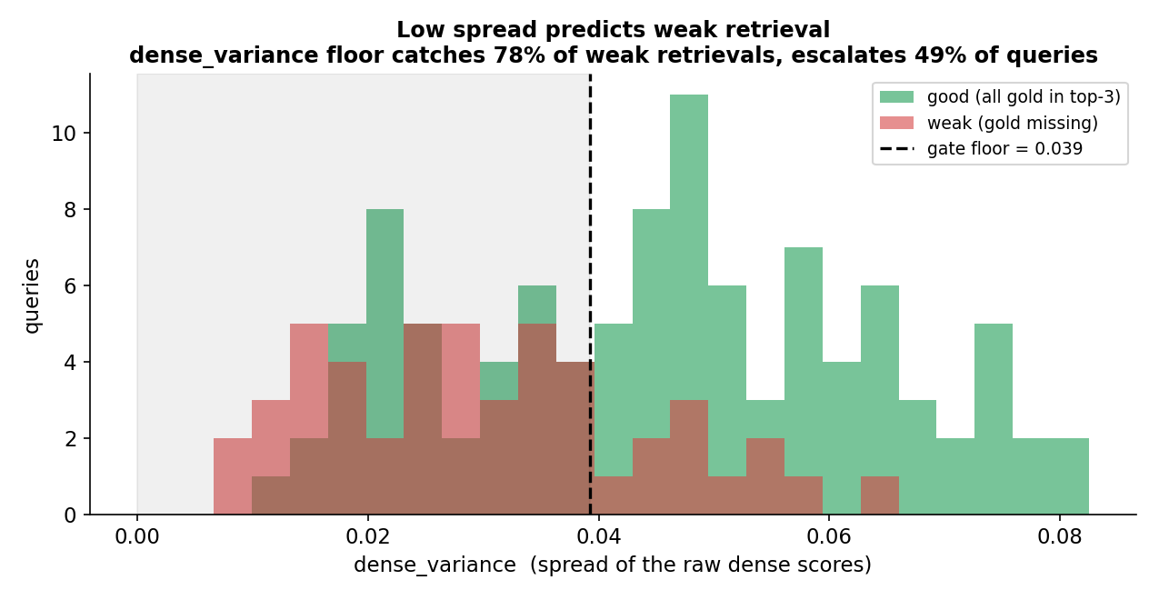
The chosen signal’s distribution for good and weak retrievals, with the calibrated floor. The shaded region escalates.
Acting on a Weak Retrieval
What you escalate to is the easy choice: rerank, rewrite, decompose, relax a filter, or hand off to a person. The gate does not care which; the expensive decision is whether, and it makes that for free on every query. The one thing escalation cannot do is invent evidence that is not in the corpus: when there is nothing to find, the win is detecting the weak retrieval and abstaining instead of answering from thin evidence. A runnable example wires the gate into a full self-correcting loop.
Adapt This to Your Corpus
The winners here are not portable; the recipe is:
- Define the window and the evidence each query needs.
- Label weak retrievals on a calibration split.
- Benchmark the cheap signals; keep what separates, drop the redundant.
- Threshold the winner into a gate, and escalate only when it fires.
Retrieval quality is observable from cheap statistics of the result, but only when the failure is one those statistics can see. Measure which signal that is on your own data.
Adjacent Work
This sits alongside corrective and adaptive retrieval. The difference is where the decision comes from: a cheap statistic of what was already retrieved, no extra model call, nothing to train.
- Query performance prediction has many post-retrieval predictors; how far the cheapest one transfers, and where it caps, is the question here.
- CRAG trains a retrieval evaluator and Self-RAG fine-tunes the generator to critique its own context; both put a trained model where this uses a free statistic.
- Adaptive-RAG routes on query complexity before retrieving, the question-shape approach this article argues against: gate on the evidence you got back, not the shape of the question.
- Sufficient-context work asks the same “is this enough?” question with an LLM judge rather than a free signal.
The full loop, corrective actions, and evaluation harness are in the self-correcting retrieval loops workshop. For the building blocks it escalates to, see late interaction models, hybrid search, and query decomposition.