
Qdrant under the hood: Product Quantization
Qdrant 1.1.0 brought the support of Scalar Quantization,
a technique of reducing the memory footprint by even four times, by using int8 to represent
the values that would be normally represented by float32.
The memory usage in vector search might be reduced even further! Please welcome Product Quantization, a brand-new feature of Qdrant 1.2.0!
Product Quantization
Product Quantization converts floating-point numbers into integers like every other quantization method. However, the process is slightly more complicated than Scalar Quantization and is more customizable, so you can find the sweet spot between memory usage and search precision. This article covers all the steps required to perform Product Quantization and the way it’s implemented in Qdrant.
Let’s assume we have a few vectors being added to the collection and that our optimizer decided to start creating a new segment.
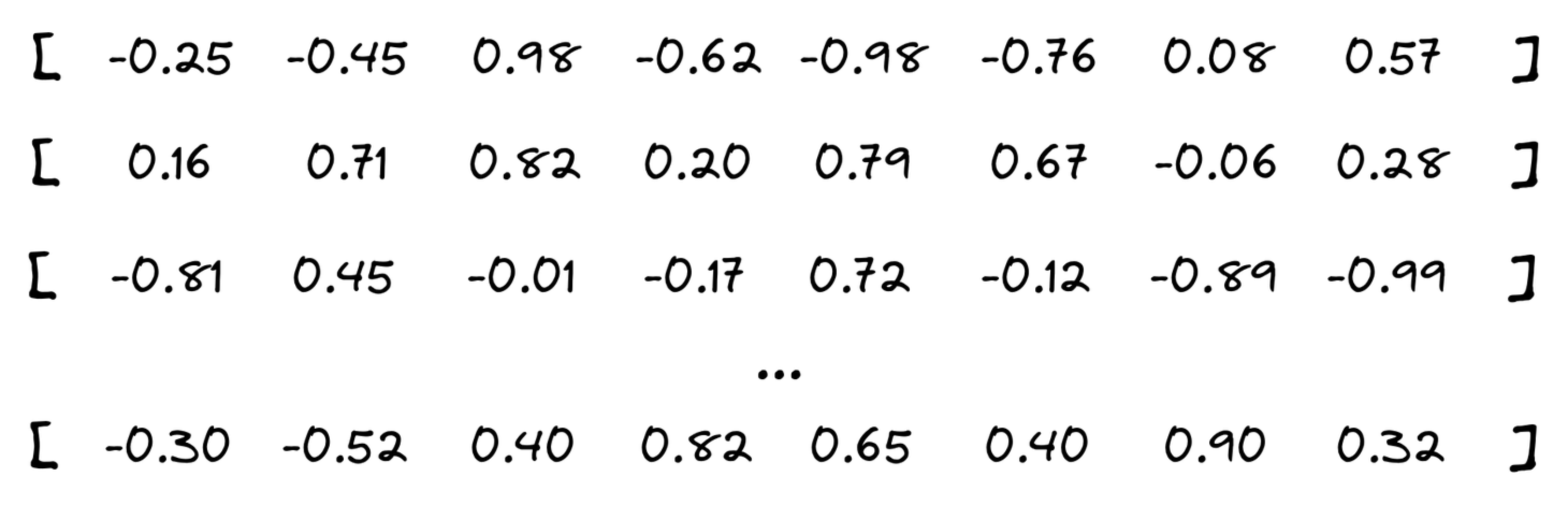
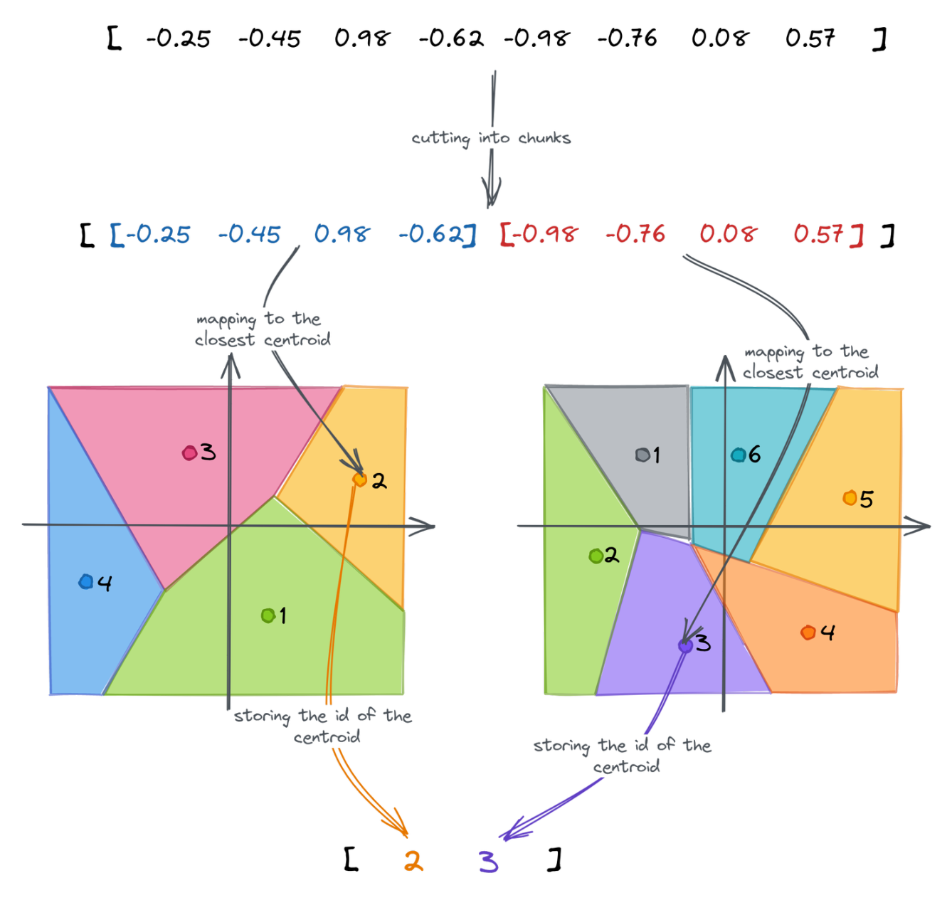
Cutting the vector into pieces
First of all, our vectors are going to be divided into chunks aka subvectors. The number of chunks is configurable, but as a rule of thumb - the lower it is, the higher the compression rate. That also comes with reduced search precision, but in some cases, you may prefer to keep the memory usage as low as possible.
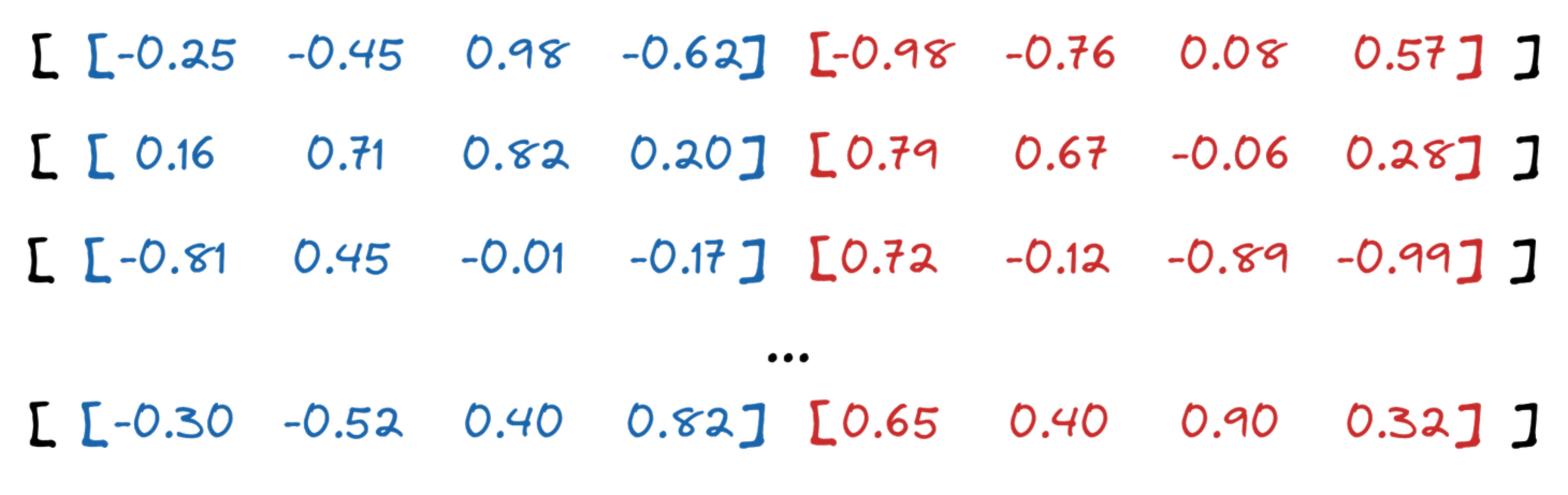
Qdrant API allows choosing the compression ratio from 4x up to 64x. In our example, we selected 16x, so each subvector will consist of 4 floats (16 bytes), and it will eventually be represented by a single byte.
Clustering
The chunks of our vectors are then used as input for clustering. Qdrant uses the K-means algorithm, with $ K = 256 $. It was selected a priori, as this is the maximum number of values a single byte represents. As a result, we receive a list of 256 centroids for each chunk and assign each of them a unique id. The clustering is done separately for each group of chunks.
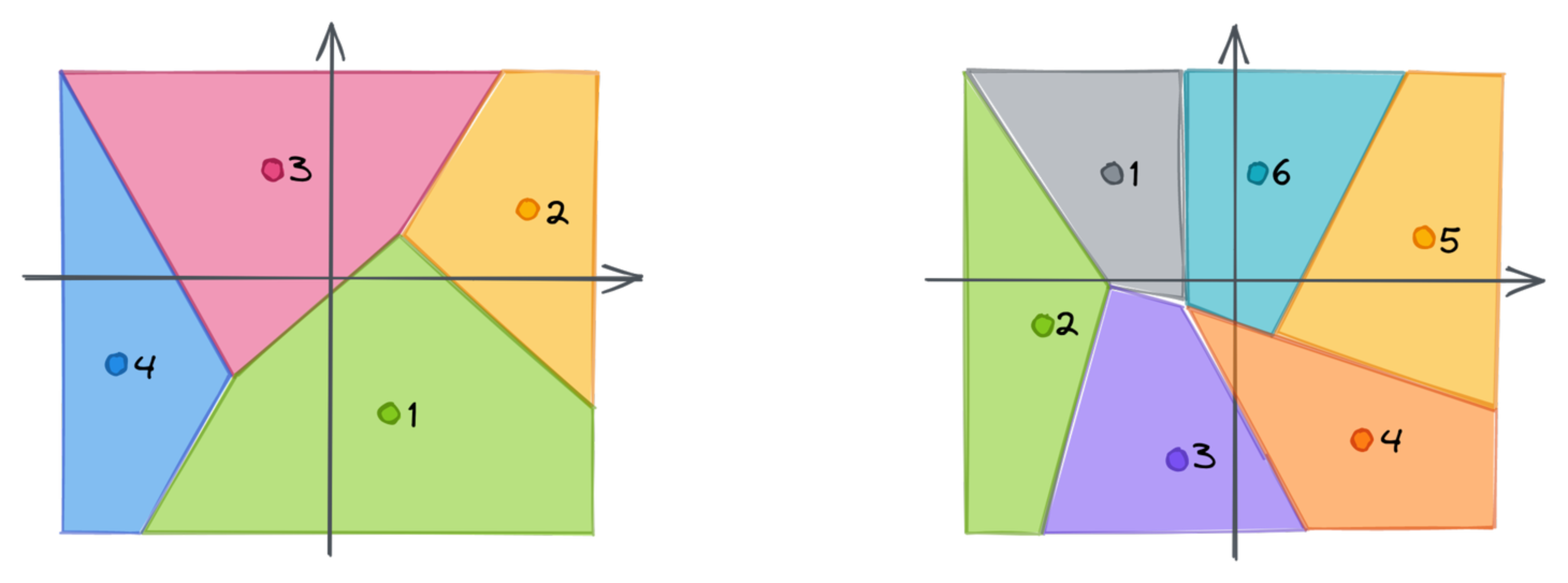
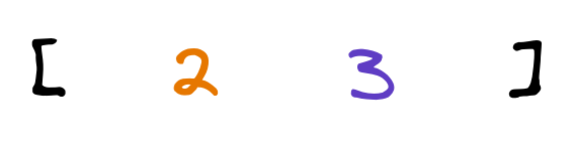
Each chunk of a vector might now be mapped to the closest centroid. That’s where we lose the precision, as a single point will only represent a whole subspace. Instead of using a subvector, we can store the id of the closest centroid. If we repeat that for each chunk, we can approximate the original embedding as a vector of subsequent ids of the centroids. The dimensionality of the created vector is equal to the number of chunks, in our case 2.
Full process
All those steps build the following pipeline of Product Quantization:
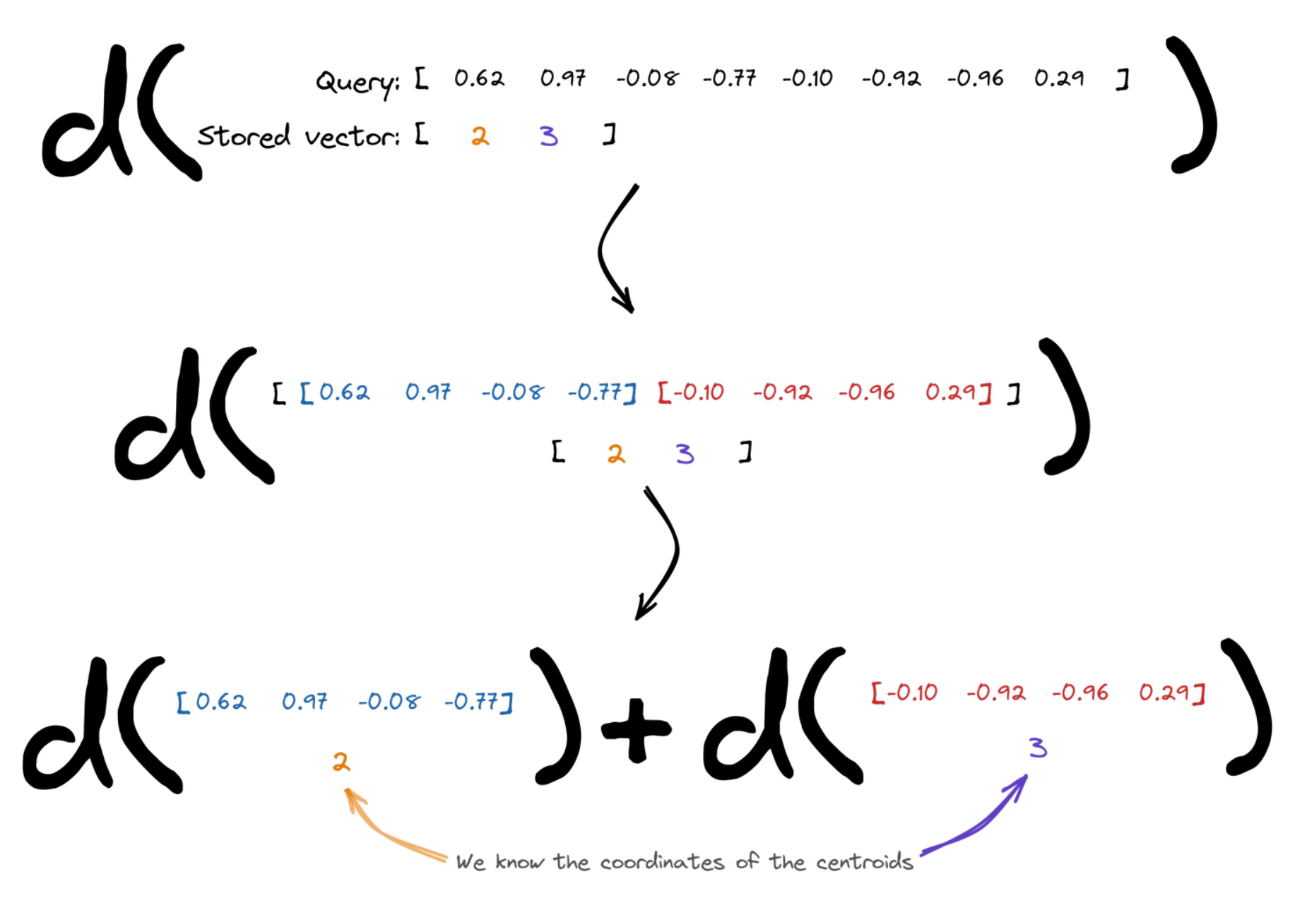
Measuring the distance
Vector search relies on the distances between the points. Enabling Product Quantization slightly changes the way it has to be calculated. The query vector is divided into chunks, and then we figure the overall distance as a sum of distances between the subvectors and the centroids assigned to the specific id of the vector we compare to. We know the coordinates of the centroids, so that’s easy.
Qdrant implementation
Search operation requires calculating the distance to multiple points. Since we calculate the distance to a finite set of centroids, those might be precomputed and reused. Qdrant creates a lookup table for each query, so it can then simply sum up several terms to measure the distance between a query and all the centroids.
| Centroid 0 | Centroid 1 | … | |
|---|---|---|---|
| Chunk 0 | 0.14213 | 0.51242 | |
| Chunk 1 | 0.08421 | 0.00142 | |
| … | … | … | … |
Benchmarks
Product Quantization comes with a cost - there are some additional operations to perform so that the performance might be reduced. However, memory usage might be reduced drastically as well. As usual, we did some benchmarks to give you a brief understanding of what you may expect.
Again, we reused the same pipeline as in the other benchmarks we published. We selected Arxiv-titles-384-angular-no-filters and Glove-100 datasets to measure the impact of Product Quantization on precision and time. Both experiments were launched with $ EF = 128 $. The results are summarized in the tables:
Glove-100
| Original | 1D clusters | 2D clusters | 3D clusters | |
|---|---|---|---|---|
| Mean precision | 0.7158 | 0.7143 | 0.6731 | 0.5854 |
| Mean search time | 2336 µs | 2750 µs | 2597 µs | 2534 µs |
| Compression | x1 | x4 | x8 | x12 |
| Upload & indexing time | 147 s | 339 s | 217 s | 178 s |
Product Quantization increases both indexing and searching time. The higher the compression ratio, the lower the search precision. The main benefit is undoubtedly the reduced usage of memory.
Arxiv-titles-384-angular-no-filters
| Original | 1D clusters | 2D clusters | 4D clusters | 8D clusters | |
|---|---|---|---|---|---|
| Mean precision | 0.9837 | 0.9677 | 0.9143 | 0.8068 | 0.6618 |
| Mean search time | 2719 µs | 4134 µs | 2947 µs | 2175 µs | 2053 µs |
| Compression | x1 | x4 | x8 | x16 | x32 |
| Upload & indexing time | 332 s | 921 s | 597 s | 481 s | 474 s |
It turns out that in some cases, Product Quantization may not only reduce the memory usage, but also the search time.
Good practices
Compared to Scalar Quantization, Product Quantization offers a higher compression rate. However, this comes with considerable trade-offs in accuracy, and at times, in-RAM search speed.
Product Quantization tends to be favored in certain specific scenarios:
- Deployment in a low-RAM environment where the limiting factor is the number of disk reads rather than the vector comparison itself
- Situations where the dimensionality of the original vectors is sufficiently high
- Cases where indexing speed is not a critical factor
In circumstances that do not align with the above, Scalar Quantization should be the preferred choice.
Qdrant documentation on Product Quantization will help you to set and configure the new quantization for your data and achieve even up to 64x memory reduction.


