GPU-Accelerated HNSW Indexing in Qdrant

Time: 45 min	Level: Intermediate	Output: GitHub

Since Qdrant v1.13, Qdrant has supported GPU-accelerated Hierarchical Navigable Small World (HNSW) indexing on self-hosted instances. Qdrant Cloud added it as a managed option more recently, as part of the new features added to Qdrant Cloud in April 2026.

GPU acceleration speeds up HNSW index builds, which addresses a problem every team building with vector search eventually runs into: the cost of re-indexing a collection when switching to a different embedding model.

At scale, with millions or tens of millions of points, CPU-based re-indexing can be slow and expensive. It drives up search latency and slows down overall traffic, since indexing and other optimizations compete with search for the same resources. GPUs help here because they excel at massive parallelization: they run many small tasks at once, while CPUs are optimized for sequential work.

Building an HNSW index involves many small operations, mostly node and edge placement in the graph, so it benefits from GPU acceleration far more than I/O-bound work, which usually requires sequential access to files.

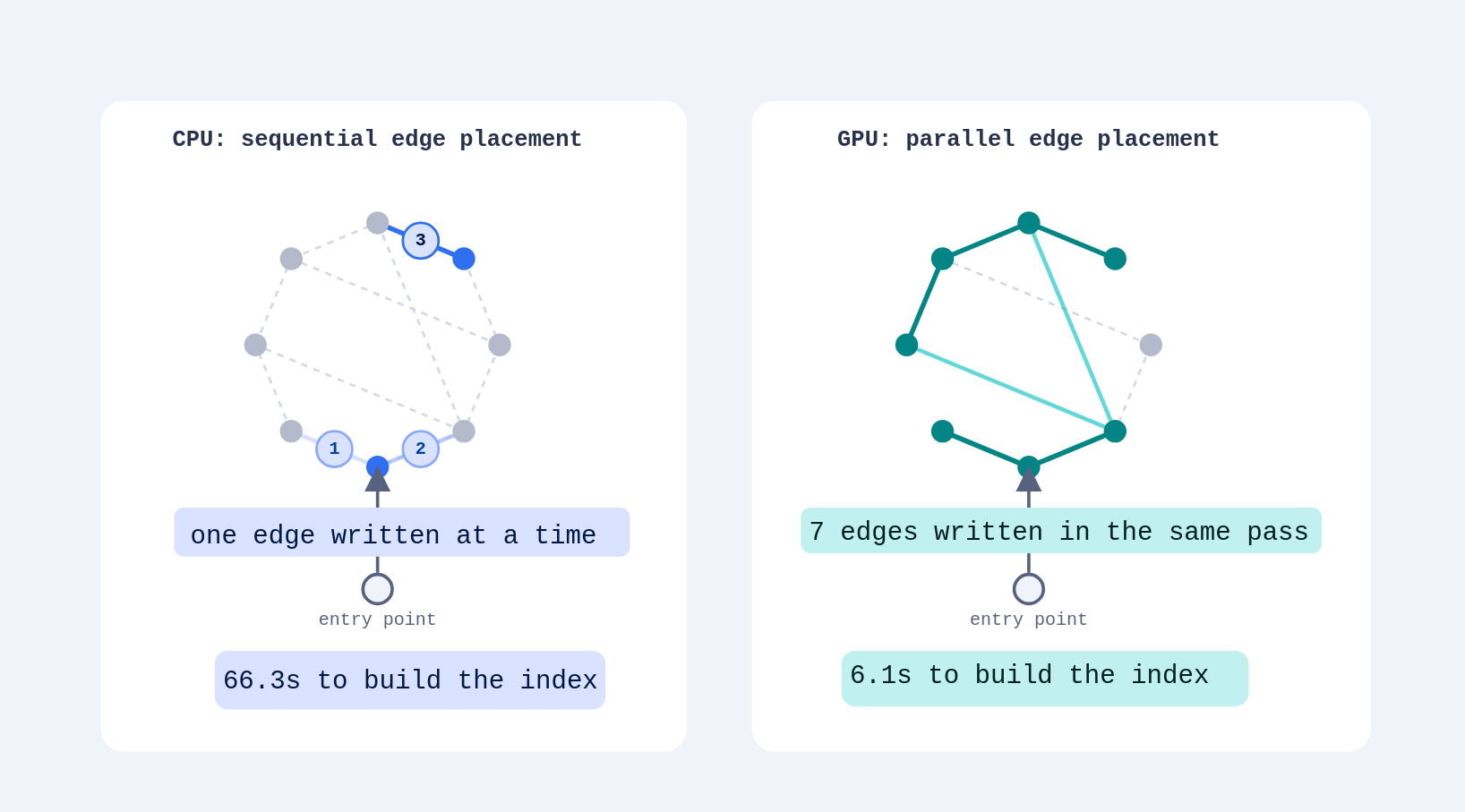
A CPU writes one HNSW edge at a time, while a GPU writes many in the same pass.

In this tutorial, you’ll set up HNSW indexing on Qdrant Cloud, measure its effect on indexing speed and query latency, compare costs with CPU index builds, and see what tradeoffs it brings.

Setting Up a GPU-Powered Cluster

You can set up a GPU-powered cluster on Qdrant Cloud either through the dedicated UI, or, as this tutorial does, with the qcloud CLI, a command-line application for managing Qdrant Cloud clusters.

Install the CLI

Install qcloud from GitHub Releases, or using go:

go install github.com/qdrant/qcloud-cli/cmd/qcloud@latest

To install from GitHub Releases instead:

curl -L https://github.com/qdrant/qcloud-cli/releases/download/v0.25.0/qcloud-linux-amd64.tar.gz | tar -xz
sudo mv qcloud /usr/local/bin/qcloud

Check the installation:

qcloud version

Authenticate and Set a Context

Create a context linked to your Qdrant Cloud account, which serves as the base for all subsequent operations.

For authentication, you need a Management API key and your account ID. Export them as environment variables:

export QDRANT_MANAGEMENT_KEY="..."
export QDRANT_ACCOUNT_ID="..."

Then create the context:

qcloud context set my-cloud \
  --api-key QDRANT_MANAGEMENT_KEY \
  --account-id QDRANT_ACCOUNT_ID

Create the Cluster

Create a GPU-powered cluster with qcloud cluster create.

Before creating the cluster, check its expected pricing given the resources you want to allocate for it and the region you want to deploy it in.

Here is an example command to create a cluster with the minimum required resources for GPUs:

qcloud cluster create \
    --disk 64GiB \
    --cloud-provider aws \
    --cloud-region us-east-1 \
    --cpu 4000m \
    --gpu 1 \
    --ram 16GiB \
    --nodes 1 \
    --disk-performance cost-optimised \
    --name "gpu-experiment"

Creating a Collection and Uploading Data

Install Dependencies

Install qdrant-client to interact with the new cluster, and huggingface-hub and polars to download and process the dataset.

pip install -q qdrant-client huggingface-hub polars

Initialize the Client

Using the credentials created for the cluster above, instantiate an asynchronous Qdrant client.

import os

from qdrant_client import AsyncQdrantClient, models

def create_qdrant_client(url: str, api_key: str) -> AsyncQdrantClient:
  return AsyncQdrantClient(
      url=url,
      api_key=api_key,
      timeout=60,
      prefer_grpc=True
  )

gpu_client = create_qdrant_client(
    os.getenv("QDRANT_URL"),
    os.getenv("QDRANT_API_KEY")
)

Prepare the Dataset

Download the ashraq/cohere-wiki-embedding-100k dataset, containing 100,000 pre-embedded Wikipedia passages.

from huggingface_hub import snapshot_download
import polars as pl

data_path = snapshot_download(
    repo_id="ashraq/cohere-wiki-embedding-100k",
    repo_type="dataset",
    allow_patterns=["data/train-*-of-*.parquet"],
)
data = pl.read_parquet(
    source=f"{data_path}/data/train-*-of-*.parquet",
    columns=["emb"]
)

Create the Collection

Create a collection with a single dense vector field and disable indexing until the upload finishes, by setting indexing_threshold above the total size (in KB) of the data you’re about to upload. This keeps the initial upload fast, since Qdrant won’t build (and rebuild) the HNSW graph while points are still streaming in.

hnsw_config.m and hnsw_config.ef_construct are left as variables here so you can vary them across experiments.

HNSW_M = 32
HNSW_EF_CONSTRUCT = 128
DIMENSIONS = len(data["emb"][0])
# 1 full-precision 256-dim vector is ~1KB
# so the size of the dataset in KB is (DIMENSIONS / 256) * DATASET_SIZE.
SIZE_KB = (DIMENSIONS // 256) * data.height

async def create_collection(client: AsyncQdrantClient, collection_name: str) -> None:
  await client.create_collection(
      collection_name=collection_name,
      optimizers_config=models.OptimizersConfigDiff(
          # add a few KB to make sure the threshold isn't surpassed
          indexing_threshold=SIZE_KB + 1000,
      ),
      vectors_config={
          "dense": models.VectorParams(
              size=DIMENSIONS,
              distance=models.Distance.COSINE,
              hnsw_config=models.HnswConfigDiff(
                  m=HNSW_M,
                  ef_construct=HNSW_EF_CONSTRUCT,
              ),
          )
      },
  )

await create_collection(gpu_client, "gpu-hnsw-experiment")

Upload the Data

Upload the embeddings in batches, giving each point a random UUID.

import uuid

BATCH_SIZE = 1000

def upload_points(client: AsyncQdrantClient, collection_name: str) -> None:
  client.upload_points(
    collection_name=collection_name,
    points=(
      models.PointStruct(
        id=str(uuid.uuid4()),
        vector={"dense": row["emb"]},
      ) for row in data.iter_rows(named=True)
    ),
    batch_size=BATCH_SIZE,
  )

upload_points(gpu_client, "gpu-hnsw-experiment")

Prepare a Query Set

To measure query latency while the HNSW index is being built, set aside a random sample of the uploaded embeddings to use as query vectors.

NUM_QUERIES = 200

queries = data.sample(NUM_QUERIES)["emb"].to_list()

Monitoring Indexing and Query Latency

Enable Indexing

Now that the upload is complete, lower the indexing_threshold back to its default so Qdrant starts building the HNSW graph.

async def enable_indexing(client: AsyncQdrantClient, collection_name: str) -> None:
  await client.update_collection(
      collection_name=collection_name,
      optimizers_config=models.OptimizersConfigDiff(
          indexing_threshold=10_000,
      ),
  )

await enable_indexing(gpu_client, "gpu-hnsw-experiment")

Query While Indexing

Run two coroutines concurrently:

One polls GET /collections/{collection}/optimizations every 0.2s until every running or queued optimization has finished, recording each snapshot.
The other repeatedly queries the collection as fast as it can, recording the latency of every request.

Both stop as soon as the polling coroutine observes that indexing has finished. This lets you later correlate query latency with the state of the HNSW build.

Start with the shared imports and the model used to timestamp each optimizations snapshot:

import asyncio
import time

from collections.abc import AsyncGenerator
from pydantic import BaseModel

MAX_POLLING_ITERATIONS = 14_400  # 14_400 its x 0.5 s/it = 7200s (2hr)
QUERY_LIMIT = 10


class OptimizationProgress(BaseModel):
    response: models.OptimizationsResponse
    timestamp: float

Poll for Optimizations

poll_for_optimizations is an async generator that yields timestamped snapshots of a collection’s running/queued optimizations and segment count on each iteration.

Since Qdrant’s idle state can briefly flicker between optimization runs, the loop waits for 5 consecutive idle snapshots (~1s at the 0.2s polling interval) before signaling completion. A max_iterations cap limits polling to 2 hours, after which the function raises TimeoutError rather than looping indefinitely.

async def poll_for_optimizations(
    client: AsyncQdrantClient,
    collection_name: str,
    signal: asyncio.Event,
    max_iterations: int = MAX_POLLING_ITERATIONS
) -> AsyncGenerator[OptimizationProgress]:
    iterations = 0
    idle_its = 0
    while iterations < max_iterations:
        optimizations, coll_info = await asyncio.gather(client.get_optimizations(
            collection_name=collection_name, _with="completed,queued,idle_segments"
        ), client.get_collection(collection_name=collection_name))
        yield OptimizationProgress(response=optimizations, timestamp=time.time())
        if len(optimizations.running) == 0 and len(optimizations.queued or []) == 0 and optimizations.summary.idle_segments == coll_info.segments_count:
            # been idle for ~1s
            if idle_its == 5:
              signal.set()
              break
            idle_its += 1
        iterations += 1
        await asyncio.sleep(0.2)
    if iterations == max_iterations:
        signal.set()
        raise TimeoutError("Operation timed out after 2 hours")

async def consume_optimizations(
    client: AsyncQdrantClient,
    collection_name: str,
    signal: asyncio.Event,
    max_iterations: int = MAX_POLLING_ITERATIONS
) -> list[OptimizationProgress]:
    optimizations = []
    async for o in poll_for_optimizations(client, collection_name, signal, max_iterations):
        optimizations.append(o)
    return optimizations

Query the Collection

query runs on its own coroutine, independent of the polling loop above. It repeatedly cycles through the queries sample built earlier, issuing one query_points request after another as fast as the client and server allow, and recording each request’s latency alongside the elapsed time since the run started. The signal event is shared with poll_for_optimizations: once that coroutine marks indexing as finished, this loop checks the same event and stops mid-cycle rather than running past the end of the experiment.

async def query(
    client: AsyncQdrantClient,
    collection_name: str,
    signal: asyncio.Event,
    queries: list[list[float]],
    limit: int = QUERY_LIMIT
) -> list[tuple[float, float]]:
    latencies = []
    start = time.time()
    while True:
        for d in queries:
            if signal.is_set():
                break
            timestamp = time.time()
            await client.query_points(
                collection_name=collection_name, query=d, limit=limit, using="dense",
            )
            finished = time.time() - timestamp
            latencies.append((timestamp - start, finished))
        if signal.is_set():
            break
    return latencies

Run Both Coroutines

Kick off consume_optimizations and query as concurrent tasks sharing the same event, wait for both to finish, then save the results to disk:

import json

OPTIMIZATIONS_FILE = "optimizations.jsonl"
LATENCIES_FILE = "latencies.jsonl"

event = asyncio.Event()
optimizations_task = asyncio.create_task(consume_optimizations(gpu_client, "gpu-hnsw-experiment", event))
query_task = asyncio.create_task(query(gpu_client, "gpu-hnsw-experiment", event, queries))
optimizations_result, latencies_result = await asyncio.gather(optimizations_task, query_task)

with open(OPTIMIZATIONS_FILE, "w") as f:
    f.writelines([r.model_dump_json() + "\n" for r in optimizations_result])

with open(LATENCIES_FILE, "w") as f:
    f.writelines(
        [
            json.dumps({"timestamp": r[0], "latency": r[1]}) + "\n"
            for r in latencies_result
        ]
    )

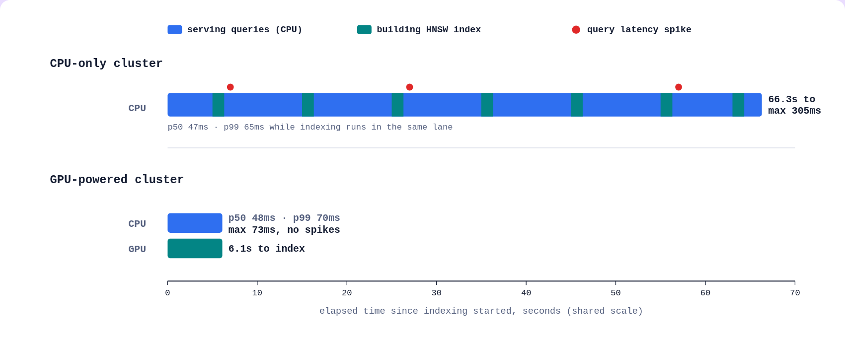
As a result of this monitoring, we expect the GPU-powered cluster to show faster optimization times, for the reasons discussed above.

Query times should be similar across both clusters, though the CPU-only cluster may show more latency spikes, since queries and optimizations compete for the same CPU cycles, increasing resource contention between reads and writes.

On the CPU-only cluster, serving queries and building the index compete for the same CPU cycles. On the GPU-accelerated cluster, the GPU builds the index on its own hardware, leaving the CPU free to serve queries.

Analyzing the Results

HNSW Indexing Time

Parse optimizations.jsonl and retrieve the starting and end time for the optimizations, then compute the total time between them.

def hnsw_indexing_time(optimizations_file: str) -> dict:
    with open(optimizations_file) as f:
        optimizations = [OptimizationProgress.model_validate_json(line.strip()) for line in f]
    full_time = optimizations[-1].timestamp - optimizations[0].timestamp
    return len(optimizations), full_time

num_recoded, full_time = hnsw_indexing_time(OPTIMIZATIONS_FILE)
print(f"Recoded {num_recoded} optimization reports.\nOptimization duration: {full_time:.2f}")

Recoded 27 optimization reports.
Optimization duration: 6.10

Query Latency Stats

Parse latencies.jsonl and compute throughput (qps) plus min, p50, p95, p99, max, and mean latency across all the queries issued while indexing was running.

from statistics import mean, quantiles

from pydantic import BaseModel


class LatencyModel(BaseModel):
    latency: float
    timestamp: float


def get_latency_stats(latency_file: str) -> dict:
    latencies: list[LatencyModel] = []
    with open(latency_file) as f:
        for line in f:
            latencies.append(LatencyModel.model_validate_json(line.strip()))
    all_time = latencies[-1].timestamp - latencies[0].timestamp
    throughput = len(latencies) / all_time  # qps
    times = [l.latency for l in latencies]
    quant_t = quantiles(times, n=100)

    return {
        "throughput": throughput,
        "min": min(times),
        "max": max(times),
        "mean": mean(times),
        "p50": quant_t[49],
        "p95": quant_t[94],
        "p99": quant_t[98],
    }


print(json.dumps(get_latency_stats(LATENCIES_FILE), indent=2))

{
  "throughput": 21.371003142800664,
  "min": 0.03345012664794922,
  "max": 0.07314538955688477,
  "mean": 0.047059608228278885,
  "p50": 0.04842805862426758,
  "p95": 0.05851303339004517,
  "p99": 0.06967230081558227
}

Comparing with CPU

Create a CPU-only cluster, with the same specifications as the one above minus the GPU, to compare against the GPU cluster.

qcloud cluster create \
    --disk 64GiB \
    --cloud-provider aws \
    --cloud-region us-east-1 \
    --cpu 4000m \
    --ram 16GiB \
    --nodes 1 \
    --disk-performance cost-optimised \
    --name "cpu-experiment"

Run the CPU cluster through the same steps used for the GPU-powered cluster:

cpu_client = create_qdrant_client(
    os.getenv("QDRANT_URL"),
    os.getenv("QDRANT_API_KEY")
)

# create collection -> upload points -> re-enable indexing
await create_collection(cpu_client, "cpu-hnsw-experiment")
upload_points(cpu_client, "cpu-hnsw-experiment")
await enable_indexing(cpu_client, "cpu-hnsw-experiment")

# collect optimizations and latency statistics
cpu_event = asyncio.Event()
cpu_optimizations_task = asyncio.create_task(consume_optimizations(cpu_client, "cpu-hnsw-experiment", cpu_event))
cpu_query_task = asyncio.create_task(query(cpu_client, "cpu-hnsw-experiment", cpu_event, queries))
optimizations_result, latencies_result = await asyncio.gather(cpu_optimizations_task, cpu_query_task)

# save statistics
CPU_OPTIMIZATIONS_FILE = "cpu-optimizations.jsonl"
CPU_LATENCIES_FILE = "cpu-latencies.jsonl"

with open(CPU_OPTIMIZATIONS_FILE, "w") as f:
    f.writelines([r.model_dump_json() + "\n" for r in optimizations_result])

with open(CPU_LATENCIES_FILE, "w") as f:
    f.writelines(
        [
            json.dumps({"timestamp": r[0], "latency": r[1]}) + "\n"
            for r in latencies_result
        ]
    )

# compute HNSW indexing time
num_recoded, full_time = hnsw_indexing_time(CPU_OPTIMIZATIONS_FILE)
print(f"Recoded {num_recoded} optimization reports.\nOptimization duration: {full_time:.2f}s")
# compute latencies statistics
print(json.dumps(get_latency_stats(CPU_LATENCIES_FILE), indent=2))

Recoded 277 optimization reports.
Optimization duration: 66.27s
{
  "throughput": 20.840132458186957,
  "min": 0.037625789642333984,
  "max": 0.3050253391265869,
  "mean": 0.04800858673459796,
  "p50": 0.04686164855957031,
  "p95": 0.05590367317199707,
  "p99": 0.06498237609863282
}

GPU vs. CPU Comparison

Both clusters had identical specs (16 GB RAM, 4 vCPU, 64 GB disk) and indexed the same 100,000 vectors with the same m and ef_construct, so the only variable between the two runs was the presence of a GPU.

Indexing time: the GPU cluster finished HNSW indexing in about 6.1s, while the CPU cluster took about 66.3s, roughly a 10x speedup. This matches the polling data: indexing on GPU wrapped up within 27 optimization snapshots (at a 0.2s polling interval), while the CPU run needed 277 snapshots to reach the same idle state.

HNSW indexing duration for the same 100,000-vector collection, GPU vs. CPU.

Query latency while indexing: throughput stayed nearly the same on both clusters (about 21 qps on GPU vs. about 21 qps on CPU), and so did the typical (p50) and even p95 latency.

The gap shows up at the tail: the CPU run’s max latency spiked to about 0.31s, more than 4x the GPU run’s about 0.07s max, and its p99 latency (about 0.065s) sat noticeably closer to that tail.

In other words, the CPU had to share cycles between building the index and serving queries, which occasionally stalled a request, while the GPU offloaded index construction and left query serving largely undisturbed.

Query latency percentiles measured while HNSW indexing ran, GPU vs. CPU.

For this workload, GPU-accelerated indexing cut the re-indexing window by an order of magnitude without introducing the latency spikes the CPU-only build showed. The advantage would be expected to grow with dataset size, since indexing time and CPU/query resource contention both scale with the number of points.

Cost of Indexing

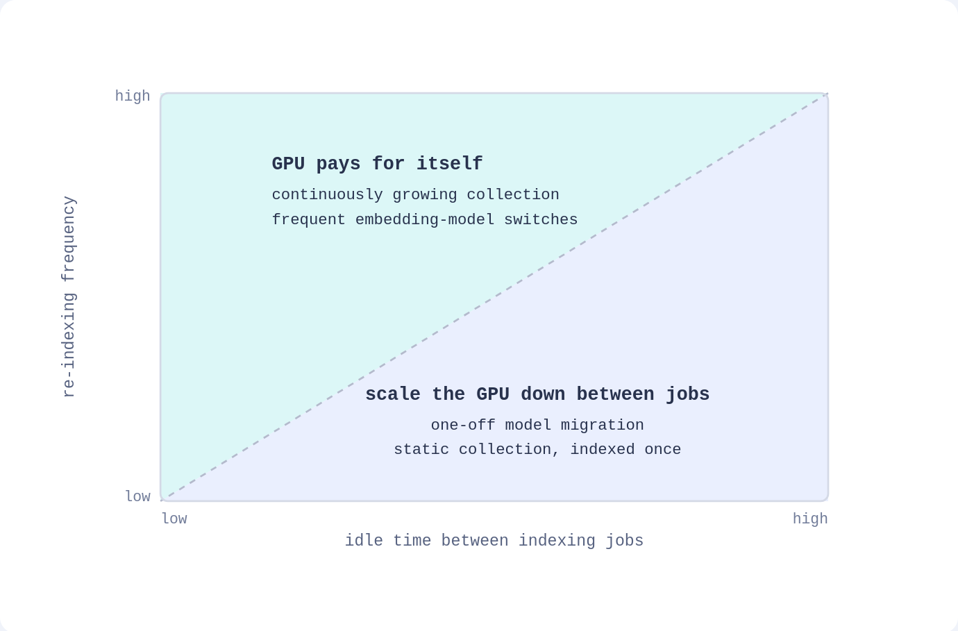
A GPU cluster tends to cost more per hour than a CPU-only cluster with equivalent specs. Whether that’s worth it depends on how much indexing you actually do with it, not on the hourly rate alone: a large enough speedup on indexing time can offset a higher hourly rate, but only for as long as the GPU is actually indexing.

It is important to consider, though, that a GPU cluster mostly pays for itself in two scenarios:

if it keeps re-indexing regularly, for example because the collection grows continuously and needs incremental re-indexing
if you switch embedding models often enough that re-indexing is a recurring cost rather than a one-off.

If neither applies, an idle GPU cluster could result in a worse deal than a CPU-only one: you might be paying the higher hourly rate with none of the speedup to offset it, since there’s no indexing work for the GPU to accelerate.

Whether GPU acceleration pays off depends on how often you re-index, not on indexing s
peed alone.