Build a Food Discovery App with Multimodal Search and Recommendations in Qdrant

Not every search journey begins with a specific destination in mind. Sometimes, you just want to explore and see what’s out there and what you might like. This is especially true when it comes to food. You might be craving something sweet, but you don’t know what. You might be also looking for a new dish to try, and you just want to see the options available. In these cases, it’s impossible to express your needs in a textual query, as the thing you are looking for is not yet defined. Qdrant’s semantic search for images is useful when you have a hard time expressing your tastes in words.

General architecture

We are happy to announce a refreshed version of our Food Discovery Demo. This time available as an open source project, so you can easily deploy it on your own and play with it. If you prefer to dive into the source code directly, then feel free to check out the GitHub repository . Otherwise, read on to learn more about the demo and how it works!

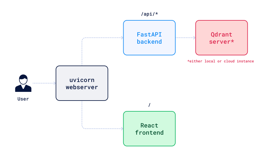
In general, our application consists of three parts: a FastAPI backend, a React frontend, and a Qdrant instance. The diagram shows how these components interact with each other:

Why did we use a CLIP model?

CLIP is a neural network that can be used to encode both images and texts into vectors. And more importantly, both images and texts are vectorized into the same latent space, so we can compare them directly. This lets you perform semantic search on images using text queries and the other way around. For example, if you search for “flat bread with toppings”, you will get images of pizza. Or if you search for “pizza”, you will get images of some flat bread with toppings, even if they were not labeled as “pizza”. This is because CLIP embeddings capture the semantics of the images and texts and can find the similarities between them no matter the wording.

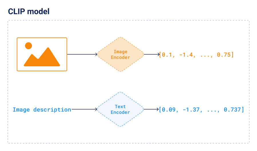
CLIP is available in many different ways. We used the pretrained clip-ViT-B-32 model available in the Sentence-Transformers library, as this is the easiest way to get started.

The dataset

The demo is based on the Wolt dataset. It contains over 2M images of dishes from different restaurants along with some additional metadata. This is how a payload for a single dish looks like (long values are shortened):

{
    "cafe": {
        "address": "VGX7+6R2 Vecchia Napoli, Valletta",
        "categories": ["italian", "pasta", "pizza", "burgers", "mediterranean"],
        "location": {"lat": 35.8980154, "lon": 14.5145106},
        "menu_id": "610936a4ee8ea7a56f4a372a",
        "name": "Vecchia Napoli Is-Suq Tal-Belt",
        "rating": 9,
        "slug": "vecchia-napoli-skyparks-suq-tal-belt"
    },
    "description": "Tomato sauce, mozzarella, guanciale, Pecorino Romano, chilli",
    "image": "https://wolt-menu-images-cdn.wolt.com/menu-images/.../amatriciana.jpeg",
    "name": "L'Amatriciana"
}

Processing this amount of records takes some time, so we precomputed the CLIP embeddings, stored them in a Qdrant collection and exported the collection as a snapshot. You may download it here.

Different search modes

The FastAPI backend exposes just a single endpoint, however it handles multiple scenarios. Let’s dive into them one by one and understand why they are needed.

Cold start

Recommendation systems struggle with a cold start problem. When a new user joins the system, there is no data about their preferences, so it’s hard to recommend anything. The same applies to our demo. When you open it, you will see a random selection of dishes, and it changes every time you refresh the page. Internally, the demo chooses some random points in the vector space.

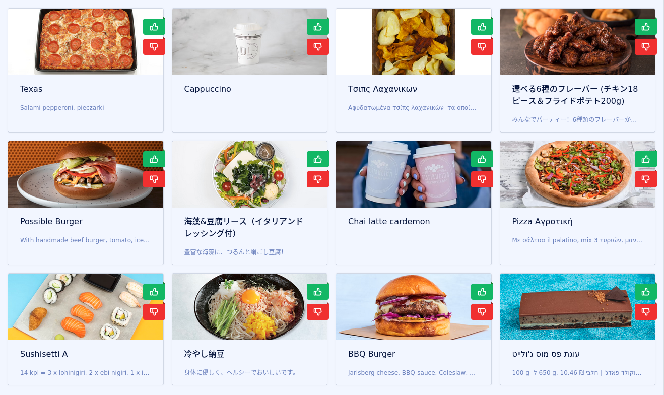
That procedure should result in returning diverse results, so we have a higher chance of showing something interesting to the user.

Textual search

Since the demo suffers from the cold start problem, we implemented a textual search mode that is useful to start exploring the data. You can type in any text query by clicking a search icon in the top right corner. The demo will use the CLIP model to encode the query into a vector and then search for the nearest neighbors in the vector space.

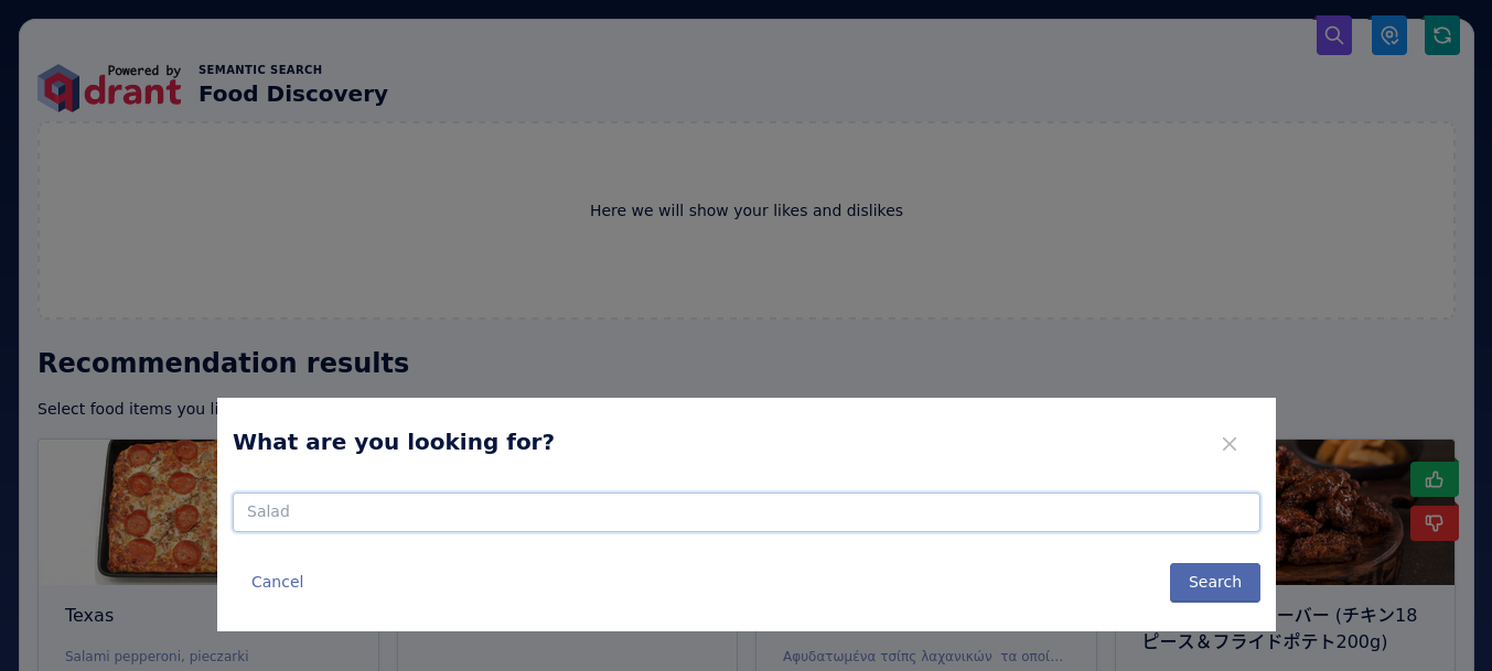
This is implemented as a group search query to Qdrant. We didn’t use a simple search, but performed grouping by the restaurant to get more diverse results. Search groups is a mechanism similar to GROUP BY clause in SQL, and it’s useful when you want to get a specific number of result per group (in our case just one).

import settings

# Encode query into a vector, model is an instance of
# sentence_transformers.SentenceTransformer that loaded CLIP model
query_vector = model.encode(query).tolist()

# Search for nearest neighbors, client is an instance of 
# qdrant_client.QdrantClient that has to be initialized before
response = client.query_points_groups(
    settings.QDRANT_COLLECTION,
    query=query_vector,
    group_by=settings.GROUP_BY_FIELD,
    group_size=1,
    limit=search_query.limit,
)

Exploring the results

The main feature of the demo is the ability to explore the space of the dishes. You can click on any of them to see more details, but first of all you can like or dislike it, and the demo will update the search results accordingly.

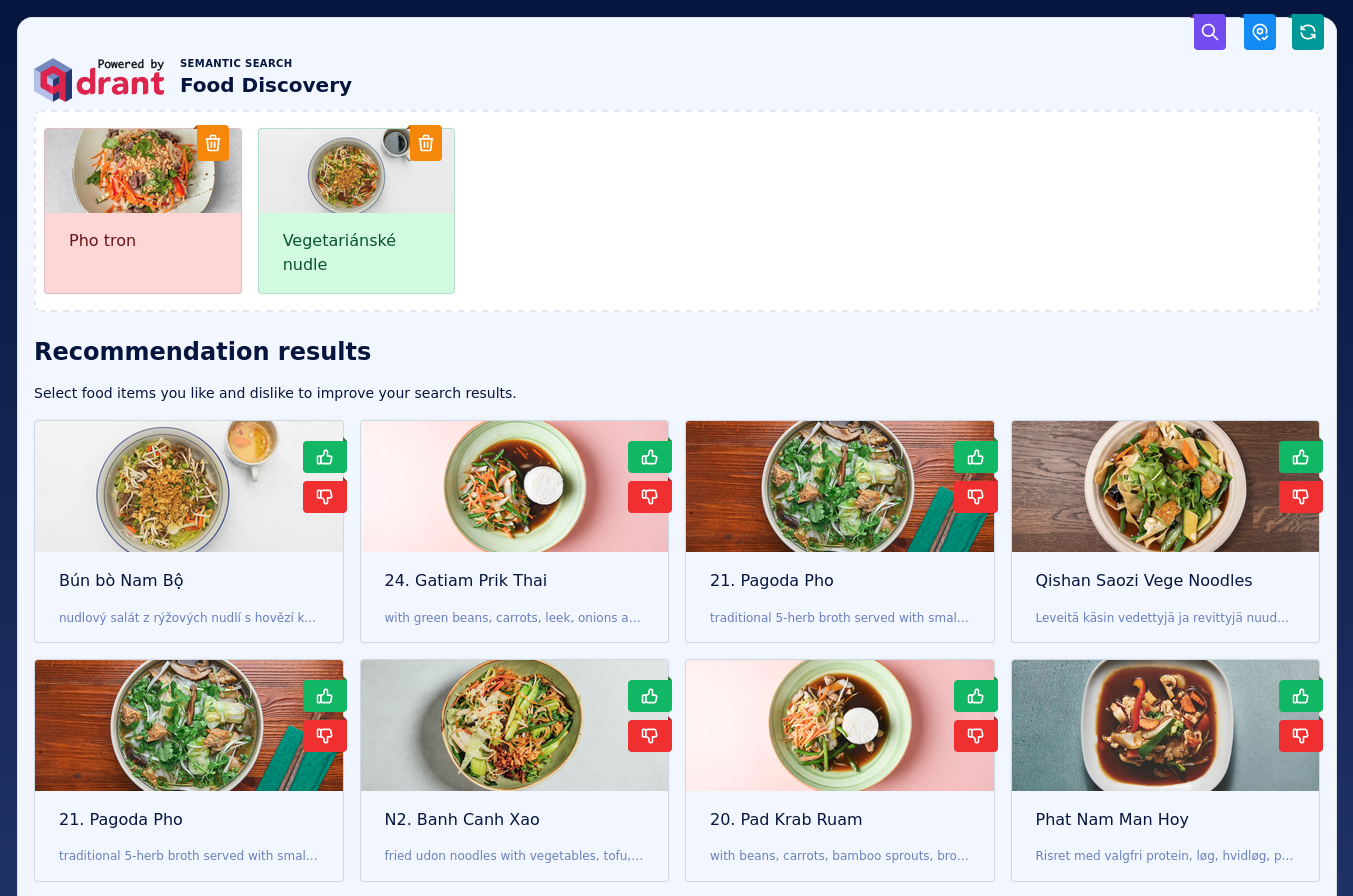
Likes and dislikes

Every like and dislike becomes a positive or a negative example for the Recommendation API. The demo calls it through the same grouped query as before, with a RecommendQuery, so the search happens server-side and the results still come back one per restaurant. The demo’s backend makes this call, with the best_score strategy as its default. The following is the same request written for the current Python client:

from qdrant_client import models

response = client.query_points_groups(
    settings.QDRANT_COLLECTION,
    query=models.RecommendQuery(
        recommend=models.RecommendInput(
            positive=search_query.positive,
            negative=search_query.negative,
            strategy=models.RecommendStrategy.BEST_SCORE,
        )
    ),
    group_by=settings.GROUP_BY_FIELD,
    group_size=1,
    limit=search_query.limit,
)

The examples can be point IDs or raw vectors, and you can mix both in one request. That is how the demo adds textual queries to a recommendation: it embeds the text with CLIP and passes the vector as one more positive example, next to the IDs of the liked dishes.

Negative feedback only

With best_score you can pass negative examples only, so a user can say “I don’t like this dish” without having to like anything first.

response = client.query_points_groups(
    settings.QDRANT_COLLECTION,
    query=models.RecommendQuery(
        recommend=models.RecommendInput(
            negative=search_query.negative,
            strategy=models.RecommendStrategy.BEST_SCORE,
        )
    ),
    group_by=settings.GROUP_BY_FIELD,
    group_size=1,
    limit=search_query.limit,
)

The default average_vector strategy still needs at least one positive example. Earlier versions of the demo worked around that by negating the mean vector of the disliked dishes and searching with it, which relies on the angle between a vector and its negation being 180 degrees under cosine distance. The best_score strategy makes that workaround unnecessary.

Choosing a recommendation strategy

The demo lets you switch between two strategies, and the difference shows how each one treats the examples. The recommendation documentation covers all strategies, including sum_scores.

average_vector is the default. It averages the positive and the negative examples into a single query vector, with the formula below, and then runs a normal search. It is as fast as a regular search, and it works with point IDs and vectors.

query = avg(positive) + (avg(positive) - avg(negative))

best_score has no single query vector. At every step of the search, it compares a candidate point with each positive and each negative example separately, and keeps the best positive score and the best negative score. If the best positive score is higher, the candidate’s score is that value, normalized with a sigmoid. Otherwise, the candidate’s score is the negated sigmoid of the best negative score, which pushes the search away from points that are closer to a negative example.

sigmoid(x) = 0.5 * (1 + x / (1 + |x|))

score = sigmoid(best_positive)     if best_positive > best_negative
score = -sigmoid(best_negative)    otherwise

Its cost grows with the number of examples, and its accuracy improves when you raise the ef search parameter.

The following observations come from the demo’s dataset and CLIP embeddings, which Qdrant 1.6 first made possible. Choosing the right strategy depends on your data, and the embeddings play a significant role, so try both on your own case.

With a single positive example, both strategies return the same results. The difference starts when you add more examples, especially negatives:

The more likes and dislikes you add, the more diverse the results of best_score get. With average_vector there is just one vector, so all the examples collapse into it, while best_score takes every example into account separately:

Passing only negatives can work as an outlier detection mechanism. The dataset was supposed to contain only food photos, but it does not. Passing food photos as negatives returns the most unlike images, which in this dataset are pill bottles and books. average_vector returns different results for the same input once it is given a positive example, so each strategy suits different questions:

Multimodality adds a catch. Text queries are far from most of the image embeddings, but close to some of them, so text-to-image search works well. When all query items come from one domain, such as only text, everything works. If you mix a positive text query with negative image examples, the best_score results are overwhelmed by the negatives, which are simply closer to the dataset embeddings. In that case, average_vector is the better choice:

Location-based search

Last but not least, location plays an important role in the food discovery process. You are definitely looking for something you can find nearby, not on the other side of the globe. Therefore, your current location can be toggled as a filtering condition. You can enable it by clicking on “Find near me” icon in the top right. This way you can find the best pizza in your neighborhood, not in the whole world. Qdrant geo radius filter is a perfect choice for this. It lets you filter the results by distance from a given point.

from qdrant_client import models

# Create a geo radius filter
query_filter = models.Filter(
    must=[
        models.FieldCondition(
            key="cafe.location",
            geo_radius=models.GeoRadius(
                center=models.GeoPoint(
                    lon=location.longitude,
                    lat=location.latitude,
                ),
                radius=location.radius_km * 1000,
            ),
        )
    ]
)

Such a filter needs a payload index to work efficiently, and it was created on a collection we used to create the snapshot. When you import it into your instance, the index will be already there.

Using the demo

The Food Discovery Demo is available online, but if you prefer to run it locally, you can do it with Docker. The README describes all the steps more in detail, but here is a quick start:

git clone git@github.com:qdrant/demo-food-discovery.git
cd demo-food-discovery
# Create .env file based on .env.example
docker-compose up -d

The demo will be available at http://localhost:8001, but you won’t be able to search anything until you import the snapshot into your Qdrant instance. If you don’t want to bother with hosting a local one, you can use the Qdrant Cloud cluster. 4 GB RAM is enough to load all the 2 million entries.

Fork and reuse

Our demo is completely open-source. Feel free to fork it, update with your own dataset or adapt the application to your use case. Whether you’re looking to understand the mechanics of semantic search or to have a foundation to build a larger project, this demo can serve as a starting point. Check out the Food Discovery Demo repository to get started. If you have any questions, feel free to reach out through Discord.