
What is Triplet Loss?
Triplet Loss was first introduced in FaceNet: A Unified Embedding for Face Recognition and Clustering in 2015, and it has been one of the most popular loss functions for supervised similarity or metric learning ever since. In its simplest explanation, Triplet Loss encourages that dissimilar pairs be distant from any similar pairs by at least a certain margin value. Mathematically, the loss value can be calculated as $L=max(d(a,p) - d(a,n) + m, 0)$, where:
- $p$, i.e., positive, is a sample that has the same label as $a$, i.e., anchor,
- $n$, i.e., negative, is another sample that has a label different from $a$,
- $d$ is a function to measure the distance between these three samples,
- and $m$ is a margin value to keep negative samples far apart.
The paper uses Euclidean distance, but it is equally valid to use any other distance metric, e.g., cosine distance.
The function has a learning objective that can be visualized as in the following:
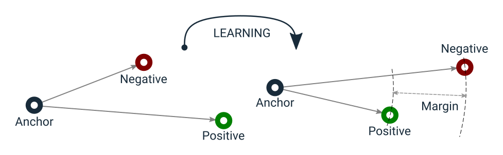
Triplet Loss learning objective
Notice that Triplet Loss does not have a side effect of urging to encode anchor and positive samples into the same point in the vector space as in Contrastive Loss. This lets Triplet Loss tolerate some intra-class variance, unlike Contrastive Loss, as the latter forces the distance between an anchor and any positive essentially to $0$. In other terms, Triplet Loss allows to stretch clusters in such a way as to include outliers while still ensuring a margin between samples from different clusters, e.g., negative pairs.
Additionally, Triplet Loss is less greedy. Unlike Contrastive Loss, it is already satisfied when different samples are easily distinguishable from similar ones. It does not change the distances in a positive cluster if there is no interference from negative examples. This is due to the fact that Triplet Loss tries to ensure a margin between distances of negative pairs and distances of positive pairs. However, Contrastive Loss takes into account the margin value only when comparing dissimilar pairs, and it does not care at all where similar pairs are at that moment. This means that Contrastive Loss may reach a local minimum earlier, while Triplet Loss may continue to organize the vector space in a better state.
Let’s demonstrate how two loss functions organize the vector space by animations. For simpler visualization, the vectors are represented by points in a 2-dimensional space, and they are selected randomly from a normal distribution.
Animation that shows how Contrastive Loss moves points in the course of training.
Animation that shows how Triplet Loss moves points in the course of training.
From mathematical interpretations of the two-loss functions, it is clear that Triplet Loss is theoretically stronger, but Triplet Loss has additional tricks that help it work better. Most importantly, Triplet Loss introduce online triplet mining strategies, e.g., automatically forming the most useful triplets.
Why triplet mining matters?
The formulation of Triplet Loss demonstrates that it works on three objects at a time:
anchor,positive- a sample that has the same label as the anchor,- and
negative- a sample with a different label from the anchor and the positive.
In a naive implementation, we could form such triplets of samples at the beginning of each epoch and then feed batches of such triplets to the model throughout that epoch. This is called “offline strategy.” However, this would not be so efficient for several reasons:
- It needs to pass $3n$ samples to get a loss value of $n$ triplets.
- Not all these triplets will be useful for the model to learn anything, e.g., yielding a positive loss value.
- Even if we form “useful” triplets at the beginning of each epoch with one of the methods that I will be implementing in this series, they may become “useless” at some point in the epoch as the model weights will be constantly updated.
Instead, we can get a batch of $n$ samples and their associated labels, and form triplets on the fly. That is called “online strategy.” Normally, this gives $n^3$ possible triplets, but only a subset of such possible triplets will be actually valid. Even in this case, we will have a loss value calculated from much more triplets than the offline strategy.
Given a triplet of (a, p, n), it is valid only if:
aandphas the same label,aandpare distinct samples,- and
nhas a different label fromaandp.
These constraints may seem to be requiring expensive computation with nested loops, but it can be efficiently implemented with tricks such as distance matrix, masking, and broadcasting. The rest of this series will focus on the implementation of these tricks.
Distance matrix
A distance matrix is a matrix of shape $(n, n)$ to hold distance values between all possible pairs made from items in two $n$-sized collections. This matrix can be used to vectorize calculations that would need inefficient loops otherwise. Its calculation can be optimized as well, and we will implement Euclidean Distance Matrix Trick (PDF) explained by Samuel Albanie. You may want to read this three-page document for the full intuition of the trick, but a brief explanation is as follows:
- Calculate the dot product of two collections of vectors, e.g., embeddings in our case.
- Extract the diagonal from this matrix that holds the squared Euclidean norm of each embedding.
- Calculate the squared Euclidean distance matrix based on the following equation: $||a - b||^2 = ||a||^2 - 2 ⟨a, b⟩ + ||b||^2$
- Get the square root of this matrix for non-squared distances.
We will implement it in PyTorch, so let’s start with imports.
import torch
import torch.nn as nn
import torch.nn.functional as F

eps = 1e-8 # an arbitrary small value to be used for numerical stability tricks
def euclidean_distance_matrix(x):
  """Efficient computation of Euclidean distance matrix

  Args:
    x: Input tensor of shape (batch_size, embedding_dim)

  Returns:
    Distance matrix of shape (batch_size, batch_size)
  """
  # step 1 - compute the dot product

  # shape: (batch_size, batch_size)
  dot_product = torch.mm(x, x.t())

  # step 2 - extract the squared Euclidean norm from the diagonal

  # shape: (batch_size,)
  squared_norm = torch.diag(dot_product)

  # step 3 - compute squared Euclidean distances

  # shape: (batch_size, batch_size)
  distance_matrix = squared_norm.unsqueeze(0) - 2 * dot_product + squared_norm.unsqueeze(1)

  # get rid of negative distances due to numerical instabilities
  distance_matrix = F.relu(distance_matrix)

  # step 4 - compute the non-squared distances

  # handle numerical stability
  # derivative of the square root operation applied to 0 is infinite
  # we need to handle by setting any 0 to eps
  mask = (distance_matrix == 0.0).float()

  # use this mask to set indices with a value of 0 to eps
  distance_matrix += mask * eps

  # now it is safe to get the square root
  distance_matrix = torch.sqrt(distance_matrix)

  # undo the trick for numerical stability
  distance_matrix *= (1.0 - mask)

  return distance_matrix
Invalid triplet masking
Now that we can compute a distance matrix for all possible pairs of embeddings in a batch,
we can apply broadcasting to enumerate distance differences for all possible triplets and represent them in a tensor of shape (batch_size, batch_size, batch_size).
However, only a subset of these $n^3$ triplets are actually valid as I mentioned earlier,
and we need a corresponding mask to compute the loss value correctly.
We will implement such a helper function in three steps:
- Compute a mask for distinct indices, e.g.,
(i != j and j != k). - Compute a mask for valid anchor-positive-negative triplets, e.g.,
labels[i] == labels[j] and labels[j] != labels[k]. - Combine two masks.
def get_triplet_mask(labels):
  """compute a mask for valid triplets

  Args:
    labels: Batch of integer labels. shape: (batch_size,)

  Returns:
    Mask tensor to indicate which triplets are actually valid. Shape: (batch_size, batch_size, batch_size)
    A triplet is valid if:
    `labels[i] == labels[j] and labels[i] != labels[k]`
    and `i`, `j`, `k` are different.
  """
  # step 1 - get a mask for distinct indices

  # shape: (batch_size, batch_size)
  indices_equal = torch.eye(labels.size()[0], dtype=torch.bool, device=labels.device)
  indices_not_equal = torch.logical_not(indices_equal)
  # shape: (batch_size, batch_size, 1)
  i_not_equal_j = indices_not_equal.unsqueeze(2)
  # shape: (batch_size, 1, batch_size)
  i_not_equal_k = indices_not_equal.unsqueeze(1)
  # shape: (1, batch_size, batch_size)
  j_not_equal_k = indices_not_equal.unsqueeze(0)
  # Shape: (batch_size, batch_size, batch_size)
  distinct_indices = torch.logical_and(torch.logical_and(i_not_equal_j, i_not_equal_k), j_not_equal_k)

  # step 2 - get a mask for valid anchor-positive-negative triplets

  # shape: (batch_size, batch_size)
  labels_equal = labels.unsqueeze(0) == labels.unsqueeze(1)
  # shape: (batch_size, batch_size, 1)
  i_equal_j = labels_equal.unsqueeze(2)
  # shape: (batch_size, 1, batch_size)
  i_equal_k = labels_equal.unsqueeze(1)
  # shape: (batch_size, batch_size, batch_size)
  valid_indices = torch.logical_and(i_equal_j, torch.logical_not(i_equal_k))

  # step 3 - combine two masks
  mask = torch.logical_and(distinct_indices, valid_indices)

  return mask
Batch-all strategy for online triplet mining
Now we are ready for actually implementing Triplet Loss itself. Triplet Loss involves several strategies to form or select triplets, and the simplest one is to use all valid triplets that can be formed from samples in a batch. This can be achieved in four easy steps thanks to utility functions we’ve already implemented:
- Get a distance matrix of all possible pairs that can be formed from embeddings in a batch.
- Apply broadcasting to this matrix to compute loss values for all possible triplets.
- Set loss values of invalid or easy triplets to $0$.
- Average the remaining positive values to return a scalar loss.
I will start by implementing this strategy, and more complex ones will follow as separate posts.
class BatchAllTtripletLoss(nn.Module):
  """Uses all valid triplets to compute Triplet loss

  Args:
    margin: Margin value in the Triplet Loss equation
  """
  def __init__(self, margin=1.):
    super().__init__()
    self.margin = margin

  def forward(self, embeddings, labels):
    """computes loss value.

    Args:
      embeddings: Batch of embeddings, e.g., output of the encoder. shape: (batch_size, embedding_dim)
      labels: Batch of integer labels associated with embeddings. shape: (batch_size,)

    Returns:
      Scalar loss value.
    """
    # step 1 - get distance matrix
    # shape: (batch_size, batch_size)
    distance_matrix = euclidean_distance_matrix(embeddings)

    # step 2 - compute loss values for all triplets by applying broadcasting to distance matrix

    # shape: (batch_size, batch_size, 1)
    anchor_positive_dists = distance_matrix.unsqueeze(2)
    # shape: (batch_size, 1, batch_size)
    anchor_negative_dists = distance_matrix.unsqueeze(1)
    # get loss values for all possible n^3 triplets
    # shape: (batch_size, batch_size, batch_size)
    triplet_loss = anchor_positive_dists - anchor_negative_dists + self.margin

    # step 3 - filter out invalid or easy triplets by setting their loss values to 0

    # shape: (batch_size, batch_size, batch_size)
    mask = get_triplet_mask(labels)
    triplet_loss *= mask
    # easy triplets have negative loss values
    triplet_loss = F.relu(triplet_loss)

    # step 4 - compute scalar loss value by averaging positive losses
    num_positive_losses = (triplet_loss > eps).float().sum()
    triplet_loss = triplet_loss.sum() / (num_positive_losses + eps)

    return triplet_loss
Conclusion
I mentioned that Triplet Loss is different from Contrastive Loss not only mathematically but also in its sample selection strategies, and I implemented the batch-all strategy for online triplet mining in this post efficiently by using several tricks.
There are other more complicated strategies such as batch-hard and batch-semihard mining, but their implementations, and discussions of the tricks I used for efficiency in this post, are worth separate posts of their own.
The future posts will cover such topics and additional discussions on some tricks to avoid vector collapsing and control intra-class and inter-class variance.