Back to Machine Learning

Modern Sparse Neural Retrieval: From Theory to Practice

Evgeniya Sukhodolskaya

·

October 23, 2024

Finding enough time to study all the modern solutions while keeping your production running is rarely feasible. Dense retrievers, hybrid retrievers, late interaction… How do they work, and where do they fit best? If only we could compare retrievers as easily as products on Amazon!

We explored the most popular modern sparse neural retrieval models and broke them down for you. By the end of this article, you’ll have a clear understanding of the current landscape in sparse neural retrieval and how to navigate through complex, math-heavy research papers with sky-high NDCG scores without getting overwhelmed.

The first part of this article is theoretical, comparing different approaches used in modern sparse neural retrieval.
The second part is more practical, showing how the best model in modern sparse neural retrieval, SPLADE++, can be used in Qdrant and recommendations on when to choose sparse neural retrieval for your solutions.

Sparse Neural Retrieval: As If Keyword-Based Retrievers Understood Meaning

Keyword-based (lexical) retrievers like BM25 provide a good explainability. If a document matches a query, it’s easy to understand why: query terms are present in the document, and if these are rare terms, they are more important for retrieval.

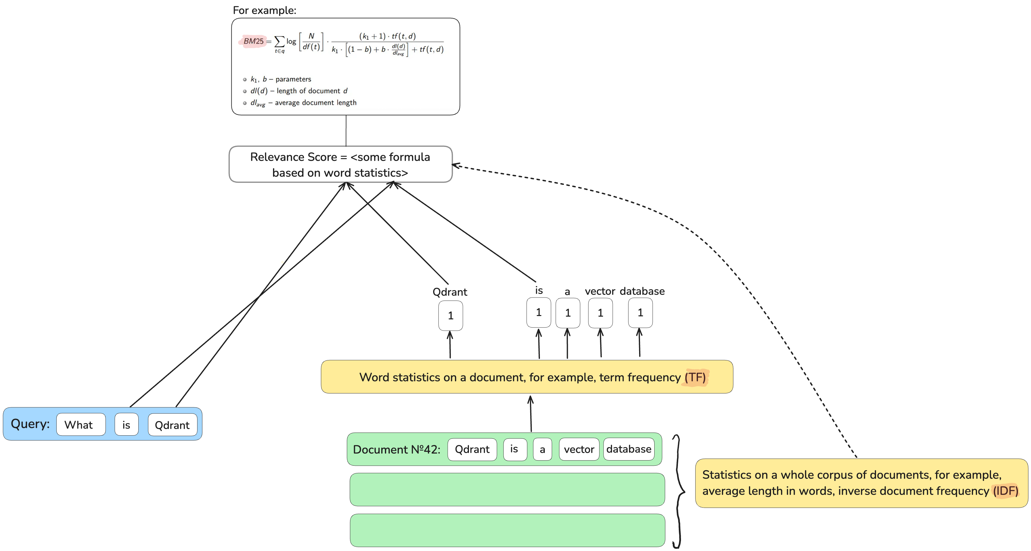
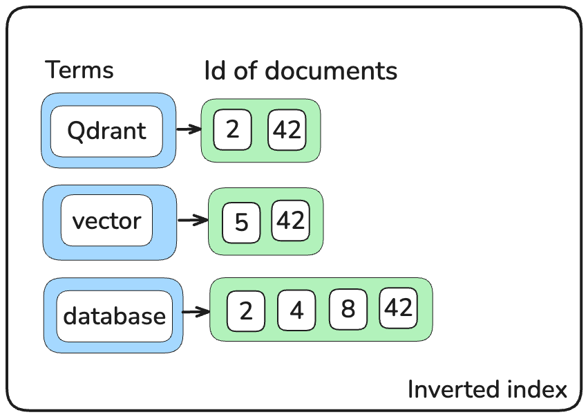
With their mechanism of exact term matching, they are super fast at retrieval. A simple inverted index, which maps back from a term to a list of documents where this term occurs, saves time on checking millions of documents.

Lexical retrievers are still a strong baseline in retrieval tasks. However, by design, they’re unable to bridge vocabulary and semantic mismatch gaps. Imagine searching for a “tasty cheese” in an online store and not having a chance to get “Gouda” or “Brie” in your shopping basket.

Dense retrievers, based on machine learning models which encode documents and queries in dense vector representations, are capable of breaching this gap and finding you “a piece of Gouda”.

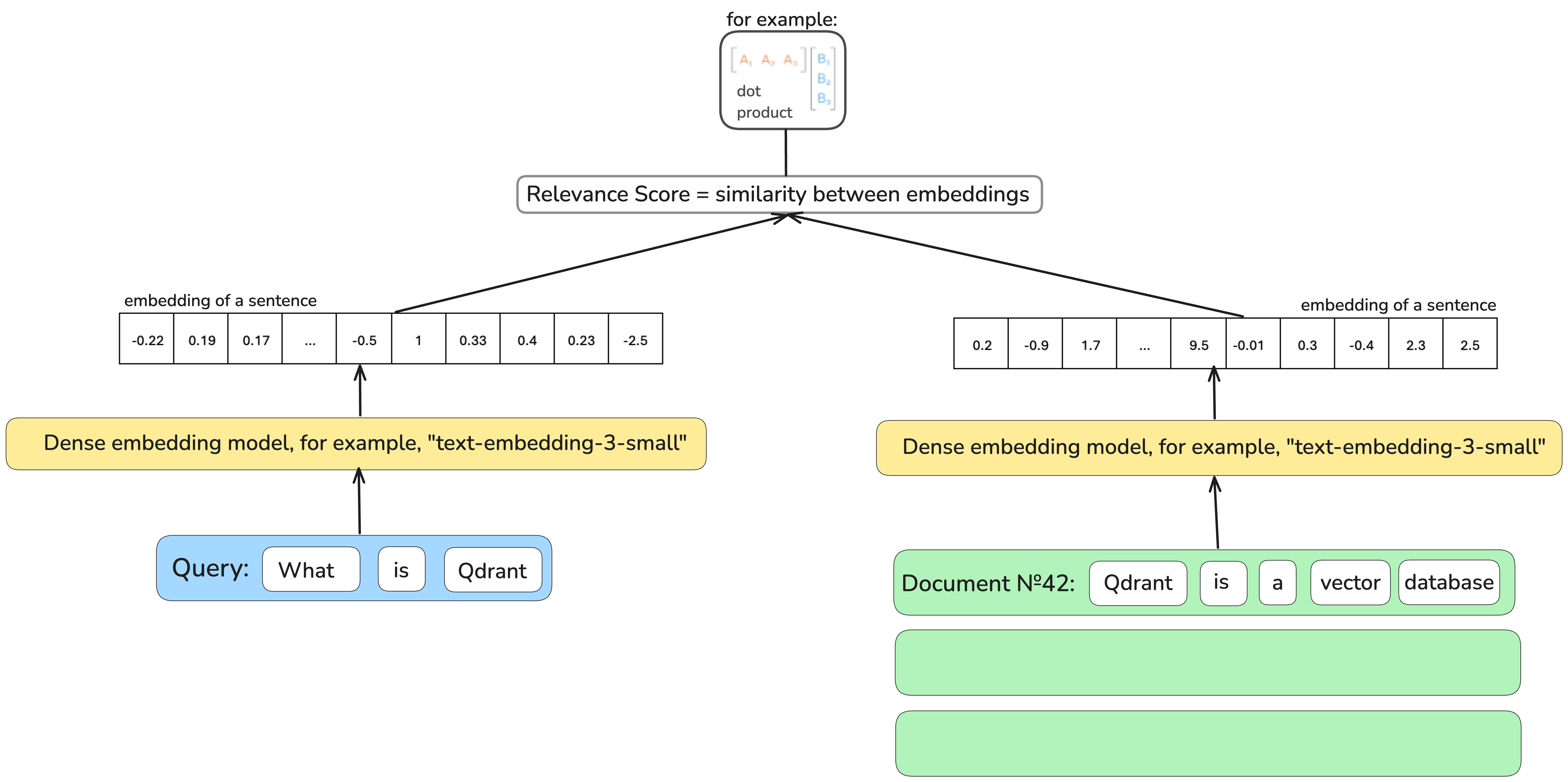
However, explainability here suffers: why is this query representation close to this document representation? Why, searching for “cheese”, we’re also offered “mouse traps”? What does each number in this vector representation mean? Which one of them is capturing the cheesiness?

Without a solid understanding, balancing result quality and resource consumption becomes challenging. Since, hypothetically, any document could match a query, relying on an inverted index with exact matching isn’t feasible. This doesn’t mean dense retrievers are inherently slower. However, lexical retrieval has been around long enough to inspire several effective architectural choices, which are often worth reusing.

Sooner or later, there should have been somebody who would say, “Wait, but what if I want something timeproof like BM25 but with semantic understanding?”

Sparse Neural Retrieval Evolution

Imagine searching for a “flabbergasting murder” story. ”Flabbergasting” is a rarely used word, so a keyword-based retriever, for example, BM25, will assign huge importance to it. Consequently, there is a high chance that a text unrelated to any crimes but mentioning something “flabbergasting” will pop up in the top results.

What if we could instead of relying on term frequency in a document as a proxy of term’s importance as it happens in BM25, directly predict a term’s importance? The goal is for rare but non-impactful terms to be assigned a much smaller weight than important terms with the same frequency, while both would be equally treated in the BM25 scenario.

How can we determine if one term is more important than another? Word impact is related to its meaning, and its meaning can be derived from its context (words which surround this particular word). That’s how dense contextual embedding models come into the picture.

All the sparse retrievers are based on the idea of taking a model which produces contextual dense vector representations for terms and teaching it to produce sparse ones. Very often, Bidirectional Encoder Representations from the Transformers (BERT) is used as a base model, and a very simple trainable neural network is added on top of it to sparsify the representations out. Training this small neural network is usually done by sampling from the MS MARCO dataset a query, relevant and irrelevant to it documents and shifting the parameters of the neural network in the direction of relevancy.

The Pioneer Of Sparse Neural Retrieval

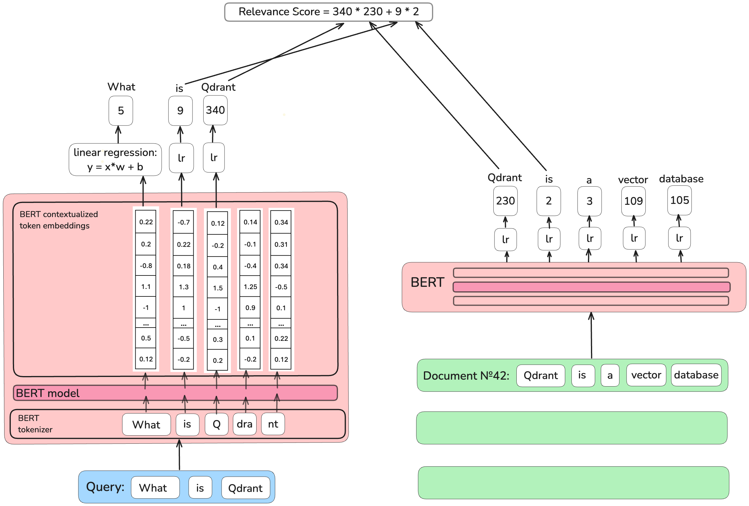The authors of one of the first sparse retrievers, the Deep Contextualized Term Weighting framework (DeepCT), predict an integer word’s impact value separately for each unique word in a document and a query. They use a linear regression model on top of the contextual representations produced by the basic BERT model, the model’s output is rounded.

When documents are uploaded into a database, the importance of words in a document is predicted by a trained linear regression model and stored in the inverted index in the same way as term frequencies in BM25 retrievers. Then, the retrieval process is identical to the BM25 one.

Why is DeepCT not a perfect solution? To train linear regression, the authors needed to provide the true value (ground truth) of each word’s importance so the model could “see” what the right answer should be. This score is hard to define in a way that it truly expresses the query-document relevancy. Which score should have the most relevant word to a query when this word is taken from a five-page document? The second relevant? The third?

Sparse Neural Retrieval on Relevance Objective

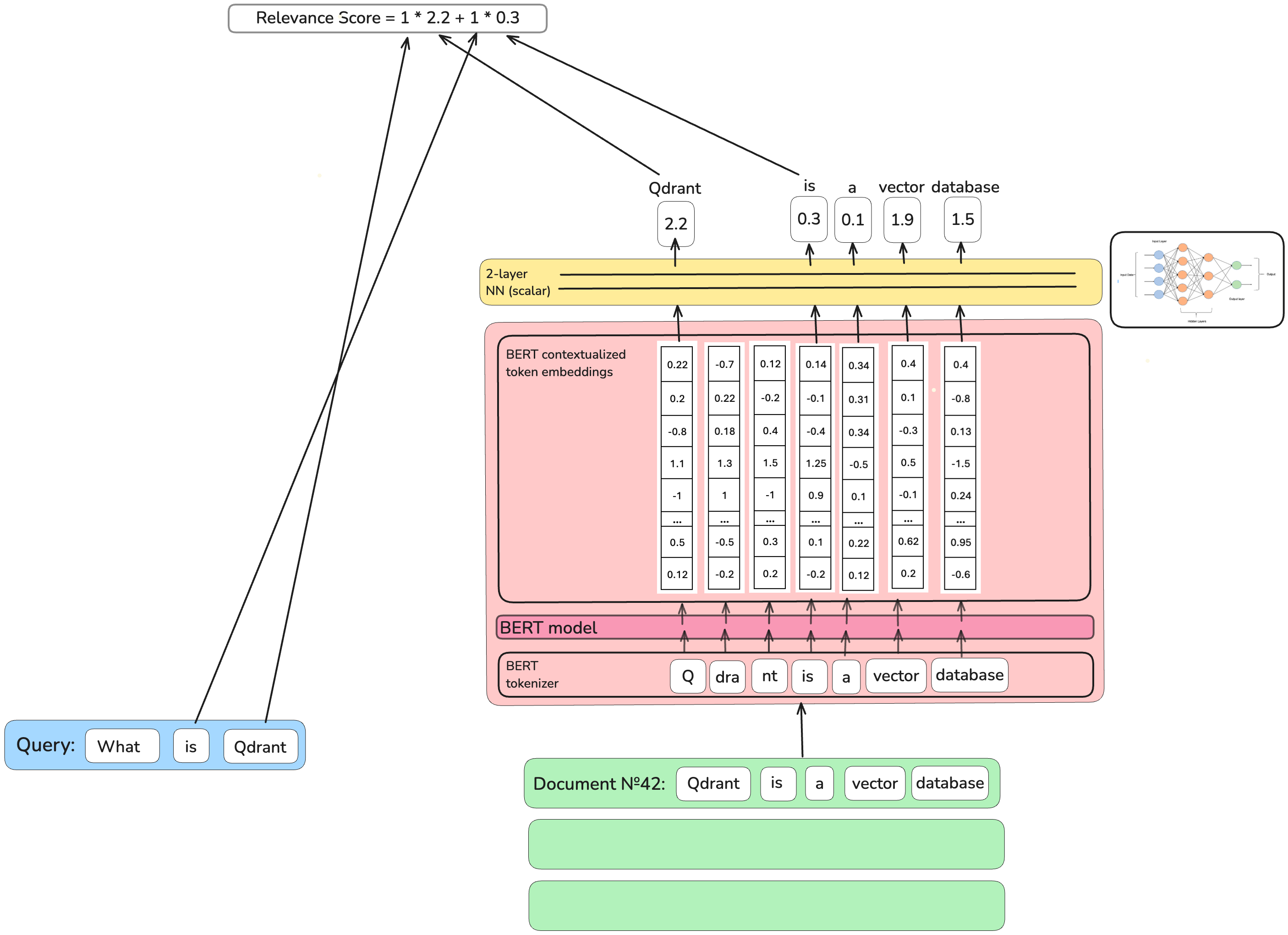It’s much easier to define whether a document as a whole is relevant or irrelevant to a query. That’s why the DeepImpact Sparse Neural Retriever authors directly used the relevancy between a query and a document as a training objective. They take BERT’s contextualized embeddings of the document’s words, transform them through a simple 2-layer neural network in a single scalar score and sum these scores up for each word overlapping with a query. The training objective is to make this score reflect the relevance between the query and the document.

Why is DeepImpact not a perfect solution? When converting texts into dense vector representations, the BERT model does not work on a word level. Sometimes, it breaks the words into parts. For example, the word “vector” will be processed by BERT as one piece, but for some words that, for example, BERT hasn’t seen before, it is going to cut the word in pieces as “Qdrant” turns to “Q”, “#dra” and “#nt”

The DeepImpact model (like the DeepCT model) takes the first piece BERT produces for a word and discards the rest. However, what can one find searching for “Q” instead of “Qdrant”?

Know Thine Tokenization

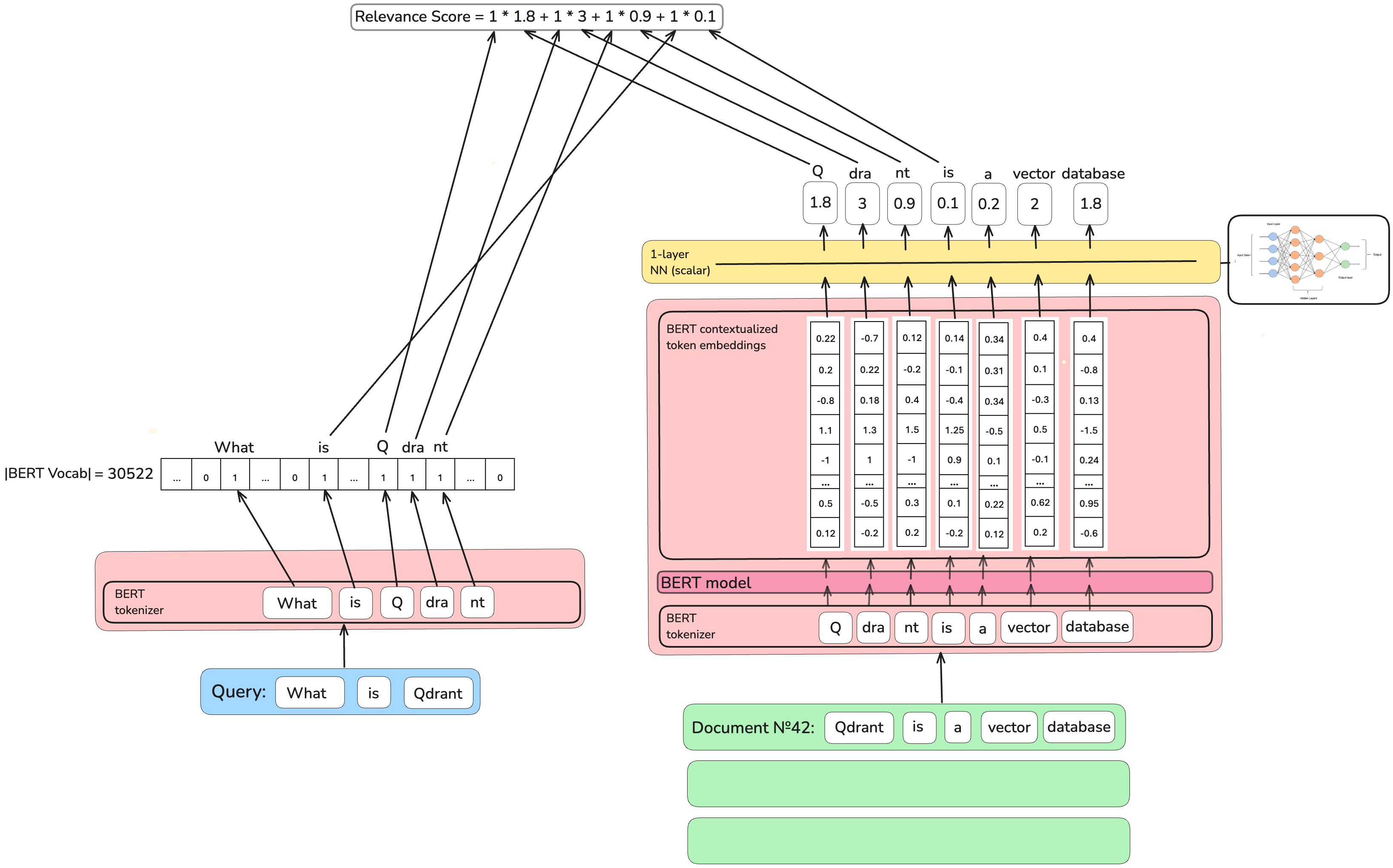To solve the problems of DeepImpact’s architecture, the Term Independent Likelihood MoDEl (TILDEv2) model generates sparse encodings on a level of BERT’s representations, not on words level. Aside from that, its authors use the identical architecture to the DeepImpact model.

Why is TILDEv2 not a perfect solution? A single scalar importance score value might not be enough to capture all distinct meanings of a word. Homonyms (pizza, cocktail, flower, and female name “Margherita”) are one of the troublemakers in information retrieval.

Sparse Neural Retriever Which Understood Homonyms

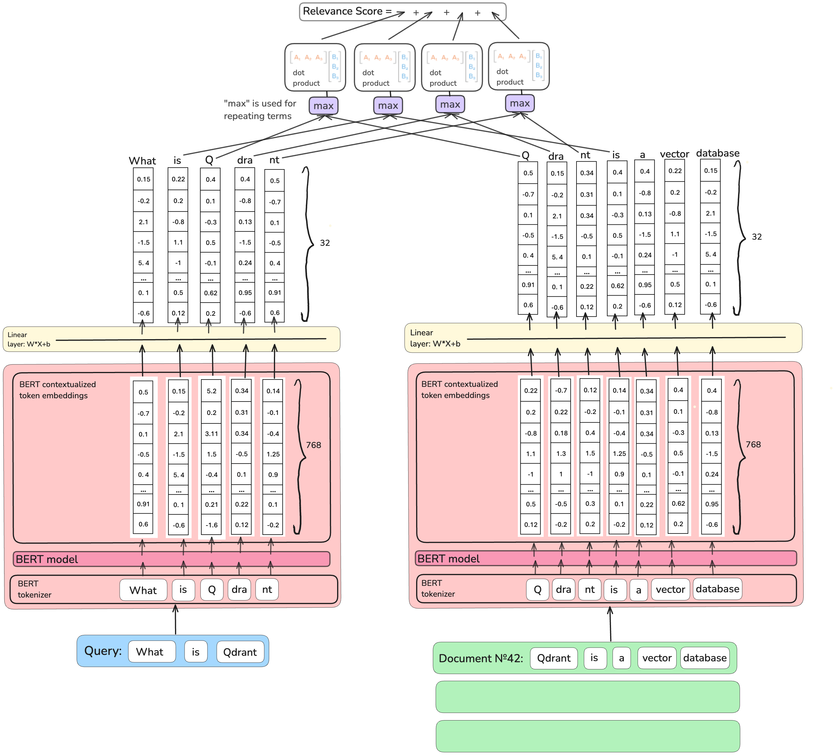
If one value for the term importance score is insufficient, we could describe the term’s importance in a vector form! Authors of the COntextualized Inverted List (COIL) model based their work on this idea. Instead of squeezing 768-dimensional BERT’s contextualised embeddings into one value, they down-project them (through the similar “relevance” training objective) to 32 dimensions. Moreover, not to miss a detail, they also encode the query terms as vectors.

For each vector representing a query token, COIL finds the closest match (using the maximum dot product) vector of the same token in a document. So, for example, if we are searching for “Revolut bank <finance institution>” and a document in a database has the sentence “Vivid bank <finance institution> was moved to the bank of Amstel <river>”, out of two “banks”, the first one will have a bigger value of a dot product with a “bank” in the query, and it will count towards the final score. The final relevancy score of a document is a sum of scores of query terms matched.

Why is COIL not a perfect solution? This way of defining the importance score captures deeper semantics; more meaning comes with more values used to describe it. However, storing 32-dimensional vectors for every term is far more expensive, and an inverted index does not work as-is with this architecture.

Back to the Roots

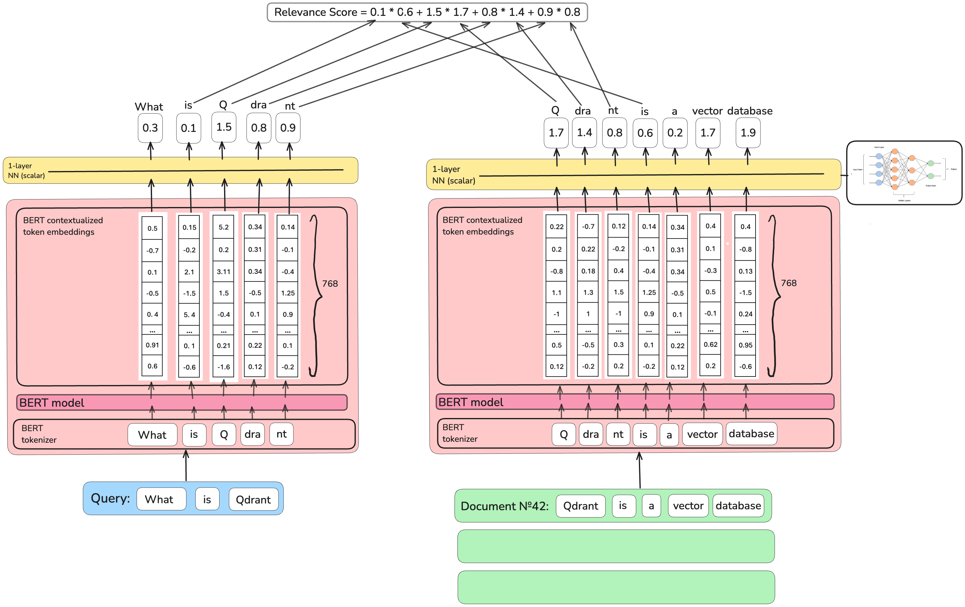
Universal COntextualized Inverted List (UniCOIL), made by the authors of COIL as a follow-up, goes back to producing a scalar value as the importance score rather than a vector, leaving unchanged all other COIL design decisions.
It optimizes resources consumption but the deep semantics understanding tied to COIL architecture is again lost.

Did we Solve the Vocabulary Mismatch Yet?

With the retrieval based on the exact matching, however sophisticated the methods to predict term importance are, we can’t match relevant documents which have no query terms in them. If you’re searching for “pizza” in a book of recipes, you won’t find “Margherita”.

A way to solve this problem is through the so-called document expansion. Let’s append words which could be in a potential query searching for this document. So, the “Margherita” document becomes “Margherita pizza”. Now, exact matching on “pizza” will work!

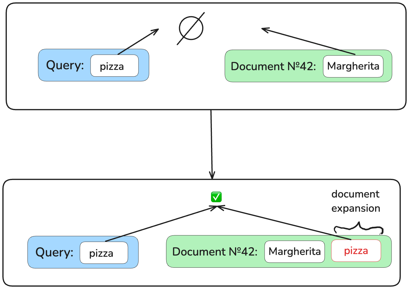
There are two types of document expansion that are used in sparse neural retrieval: external (one model is responsible for expansion, another one for retrieval) and internal (all is done by a single model).

External Document Expansion

External document expansion uses a generative model (Mistral 7B, Chat-GPT, and Claude are all generative models, generating words based on the input text) to compose additions to documents before converting them to sparse representations and applying exact matching methods.

External Document Expansion with docT5query

docT5query is the most used document expansion model. It is based on the Text-to-Text Transfer Transformer (T5) model trained to generate top-k possible queries for which the given document would be an answer. These predicted short queries (up to ~50-60 words) can have repetitions in them, so it also contributes to the frequency of the terms if the term frequency is considered by the retriever.

The problem with docT5query expansion is a very long inference time, as with any generative model: it can generate only one token per run, and it spends a fair share of resources on it.

External Document Expansion with Term Independent Likelihood MODel (TILDE)

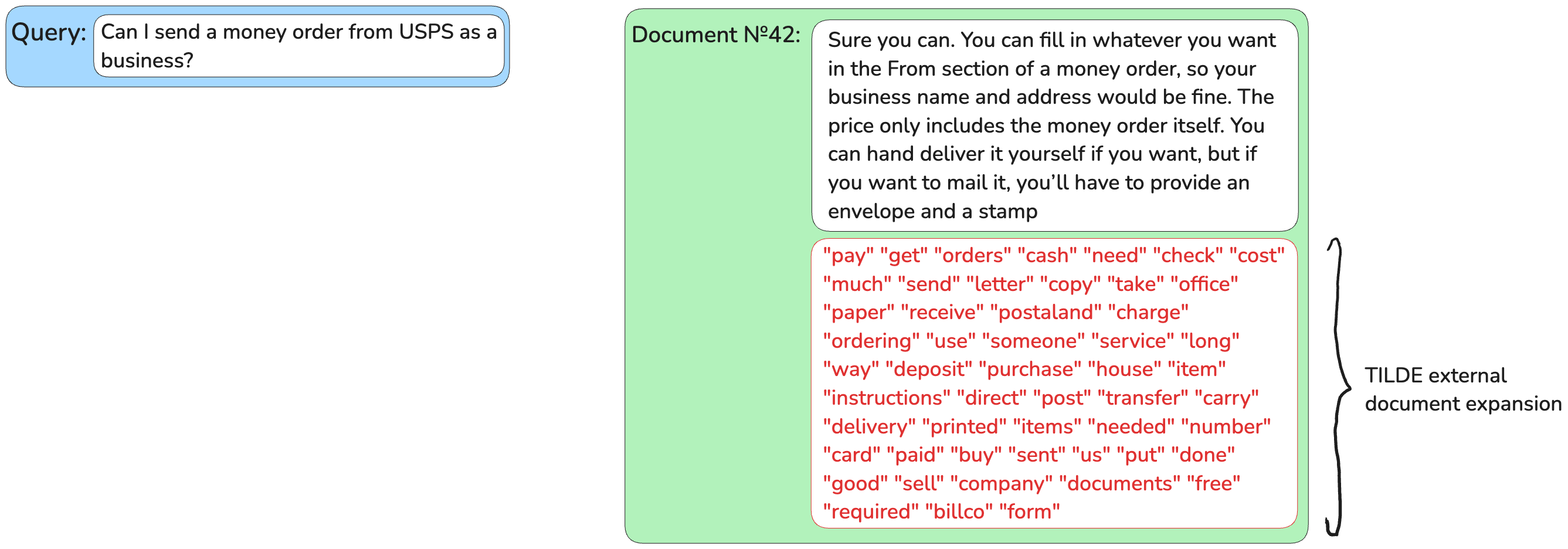
Term Independent Likelihood MODel (TILDE) is an external expansion method that reduces the passage expansion time compared to docT5query by 98%. It uses the assumption that words in texts are independent of each other (as if we were inserting in our speech words without paying attention to their order), which allows for the parallelisation of document expansion.

Instead of predicting queries, TILDE predicts the most likely terms to see next after reading a passage’s text (query likelihood paradigm). TILDE takes the probability distribution of all tokens in a BERT vocabulary based on the document’s text and appends top-k of them to the document without repetitions.

Problems of external document expansion: External document expansion might not be feasible in many production scenarios where there’s not enough time or compute to expand each and every document you want to store in a database and then additionally do all the calculations needed for retrievers. To solve this problem, a generation of models was developed which do everything in one go, expanding documents “internally”.

Internal Document Expansion

Let’s assume we don’t care about the context of query terms, so we can treat them as independent words that we combine in random order to get the result. Then, for each contextualized term in a document, we are free to pre-compute how this term affects every word in our vocabulary.

For each document, a vector of the vocabulary length is created. To fill this vector in, for each word in the vocabulary, it is checked if the influence of any document term on it is big enough to consider it. Otherwise, the vocabulary word’s score in a document vector will be zero. For example, by pre-computing vectors for the document “pizza Margherita” on a vocabulary of 50,000 most used English words, for this small document of two words, we will get a 50,000-dimensional vector of zeros, where non-zero values will be for a “pizza”, “pizzeria”, “flower”, “woman”, “girl”, “Margherita”, “cocktail” and “pizzaiolo”.

Sparse Neural Retriever with Internal Document Expansion

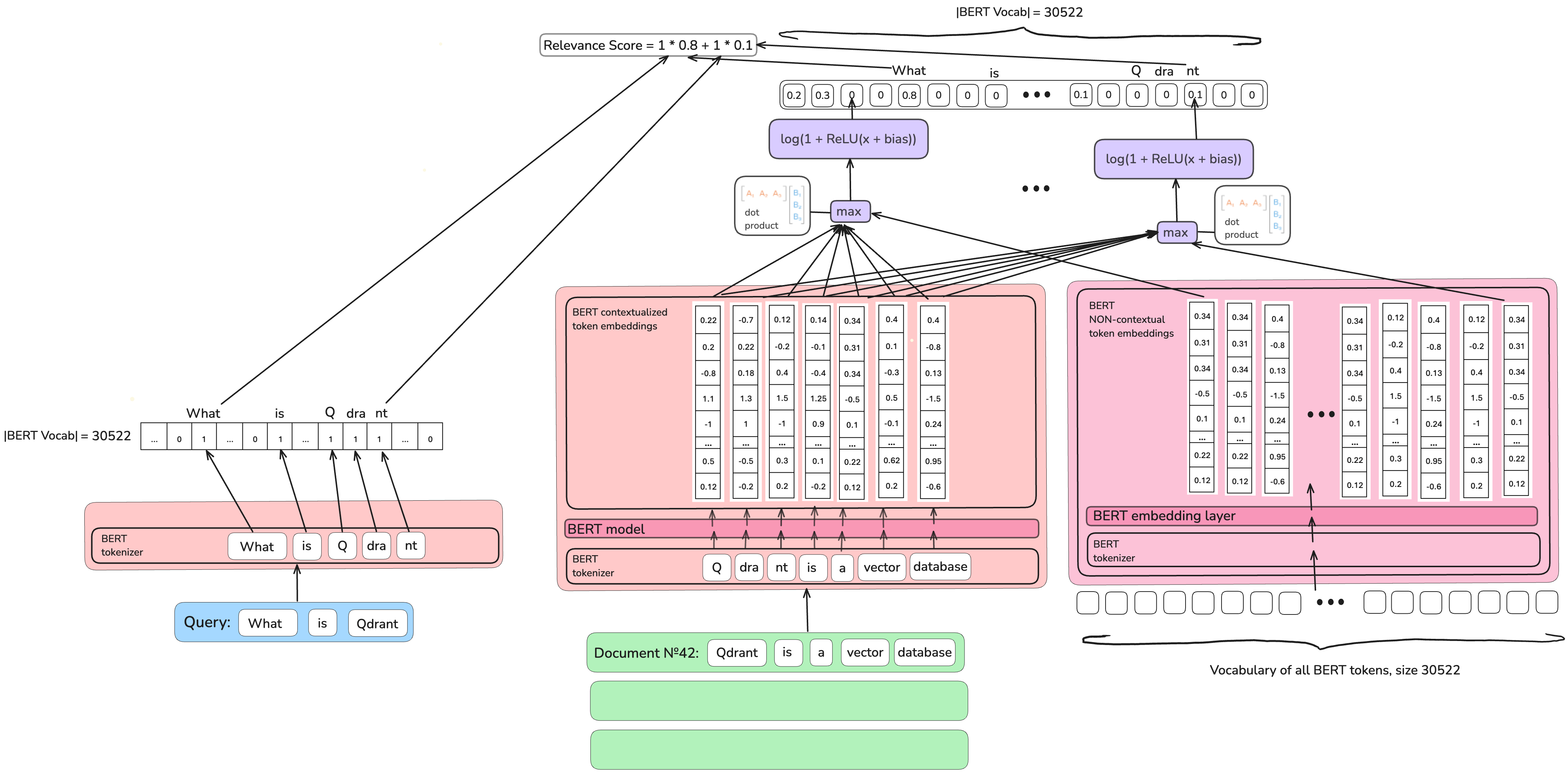
The authors of the Sparse Transformer Matching (SPARTA) model use BERT’s model and BERT’s vocabulary (around 30,000 tokens). For each token in BERT vocabulary, they find the maximum dot product between it and contextualized tokens in a document and learn a threshold of a considerable (non-zero) effect. Then, at the inference time, the only thing to be done is to sum up all scores of query tokens in that document.

Why is SPARTA not a perfect solution? Trained on the MS MARCO dataset, many sparse neural retrievers, including SPARTA, show good results on MS MARCO test data, but when it comes to generalisation (working with other data), they could perform worse than BM25.

State-of-the-Art of Modern Sparse Neural Retrieval

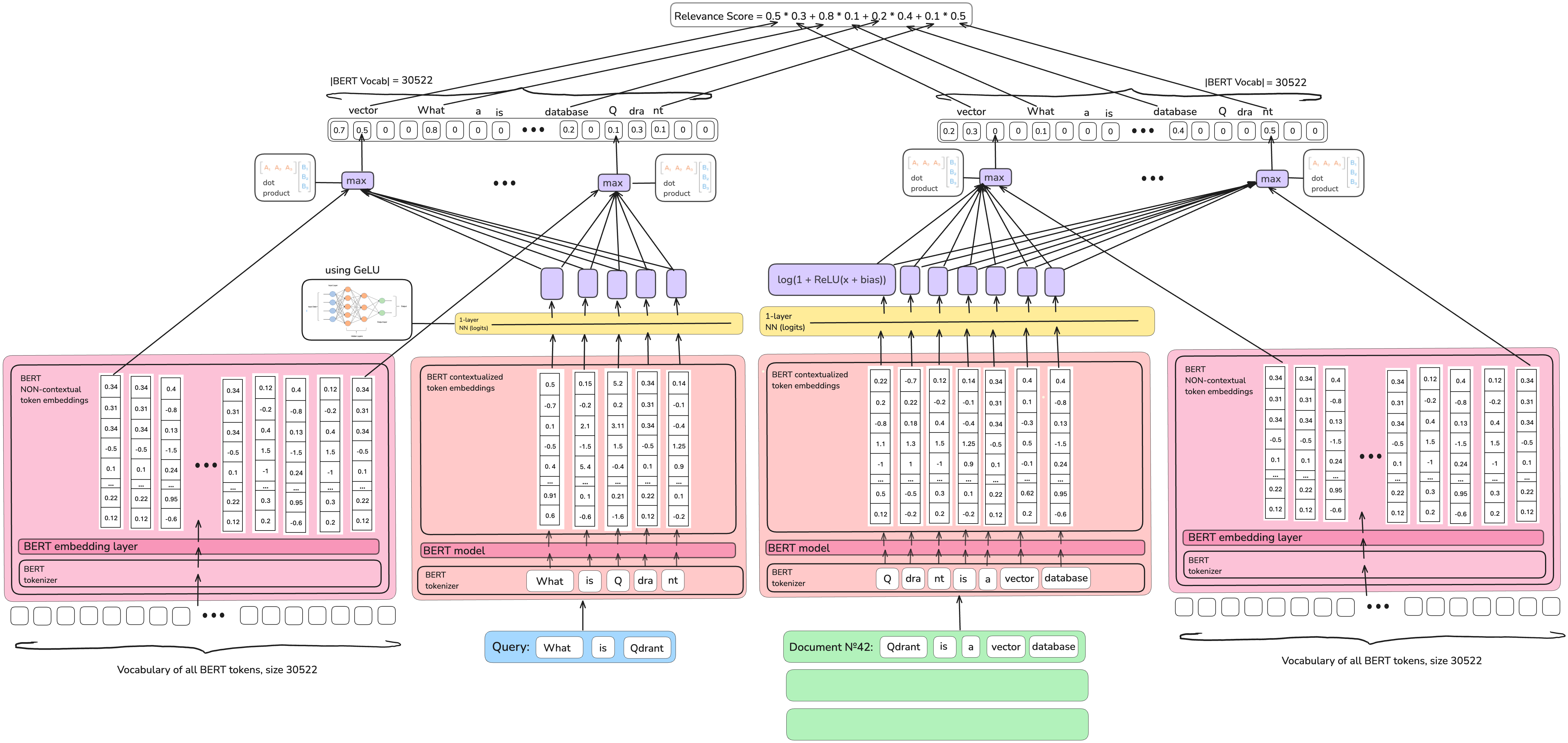The authors of the Sparse Lexical and Expansion Model (SPLADE)] family of models added dense model training tricks to the internal document expansion idea, which made the retrieval quality noticeably better.

• The SPARTA model is not sparse enough by construction, so authors of the SPLADE family of models introduced explicit sparsity regularisation, preventing the model from producing too many non-zero values.
• The SPARTA model mostly uses the BERT model as-is, without any additional neural network to capture the specifity of Information Retrieval problem, so SPLADE models introduce a trainable neural network on top of BERT with a specific architecture choice to make it perfectly fit the task.
• SPLADE family of models, finally, uses knowledge distillation, which is learning from a bigger (and therefore much slower, not-so-fit for production tasks) model how to predict good representations.

One of the last versions of the SPLADE family of models is SPLADE++.
SPLADE++, opposed to SPARTA model, expands not only documents but also queries at inference time. We’ll demonstrate this in the next section.

SPLADE++ in Qdrant

In Qdrant, you can use SPLADE++ easily with our lightweight library for embeddings called FastEmbed.

Setup

Install FastEmbed.

pip install fastembed

Import sparse text embedding models supported in FastEmbed.

from fastembed import SparseTextEmbedding

You can list all sparse text embedding models currently supported.

SparseTextEmbedding.list_supported_models()

[{'model': 'prithivida/Splade_PP_en_v1',
  'vocab_size': 30522,
  'description': 'Independent Implementation of SPLADE++ Model for English',
  'size_in_GB': 0.532,
  'sources': {'hf': 'Qdrant/SPLADE_PP_en_v1'},
  'model_file': 'model.onnx'},
 {'model': 'prithvida/Splade_PP_en_v1',
  'vocab_size': 30522,
  'description': 'Independent Implementation of SPLADE++ Model for English',
  'size_in_GB': 0.532,
  'sources': {'hf': 'Qdrant/SPLADE_PP_en_v1'},
  'model_file': 'model.onnx'},
 {'model': 'Qdrant/bm42-all-minilm-l6-v2-attentions',
  'vocab_size': 30522,
  'description': 'Light sparse embedding model, which assigns an importance score to each token in the text',
  'size_in_GB': 0.09,
  'sources': {'hf': 'Qdrant/all_miniLM_L6_v2_with_attentions'},
  'model_file': 'model.onnx',
  'additional_files': ['stopwords.txt'],
  'requires_idf': True},
 {'model': 'Qdrant/bm25',
  'description': 'BM25 as sparse embeddings meant to be used with Qdrant',
  'size_in_GB': 0.01,
  'sources': {'hf': 'Qdrant/bm25'},
  'model_file': 'mock.file',
  'additional_files': ['arabic.txt',
   'azerbaijani.txt',
   'basque.txt',
   'bengali.txt',
   'catalan.txt',
   'chinese.txt',
   'danish.txt',
   'dutch.txt',
   'english.txt',
   'finnish.txt',
   'french.txt',
   'german.txt',
   'greek.txt',
   'hebrew.txt',
   'hinglish.txt',
   'hungarian.txt',
   'indonesian.txt',
   'italian.txt',
   'kazakh.txt',
   'nepali.txt',
   'norwegian.txt',
   'portuguese.txt',
   'romanian.txt',
   'russian.txt',
   'slovene.txt',
   'spanish.txt',
   'swedish.txt',
   'tajik.txt',
   'turkish.txt'],
  'requires_idf': True}]

Load SPLADE++.

sparse_model_name = "prithivida/Splade_PP_en_v1"
sparse_model = SparseTextEmbedding(model_name=sparse_model_name)

The model files will be fetched and downloaded, with progress showing.

Embed data

We will use a toy movie description dataset.

descriptions = ["In 1431, Jeanne d'Arc is placed on trial on charges of heresy. The ecclesiastical jurists attempt to force Jeanne to recant her claims of holy visions.",
 "A film projectionist longs to be a detective, and puts his meagre skills to work when he is framed by a rival for stealing his girlfriend's father's pocketwatch.",
 "A group of high-end professional thieves start to feel the heat from the LAPD when they unknowingly leave a clue at their latest heist.",
 "A petty thief with an utter resemblance to a samurai warlord is hired as the lord's double. When the warlord later dies the thief is forced to take up arms in his place.",
 "A young boy named Kubo must locate a magical suit of armour worn by his late father in order to defeat a vengeful spirit from the past.",
 "A biopic detailing the 2 decades that Punjabi Sikh revolutionary Udham Singh spent planning the assassination of the man responsible for the Jallianwala Bagh massacre.",
 "When a machine that allows therapists to enter their patients' dreams is stolen, all hell breaks loose. Only a young female therapist, Paprika, can stop it.",
 "An ordinary word processor has the worst night of his life after he agrees to visit a girl in Soho whom he met that evening at a coffee shop.",
 "A story that revolves around drug abuse in the affluent north Indian State of Punjab and how the youth there have succumbed to it en-masse resulting in a socio-economic decline.",
 "A world-weary political journalist picks up the story of a woman's search for her son, who was taken away from her decades ago after she became pregnant and was forced to live in a convent.",
 "Concurrent theatrical ending of the TV series Neon Genesis Evangelion (1995).",
 "During World War II, a rebellious U.S. Army Major is assigned a dozen convicted murderers to train and lead them into a mass assassination mission of German officers.",
 "The toys are mistakenly delivered to a day-care center instead of the attic right before Andy leaves for college, and it's up to Woody to convince the other toys that they weren't abandoned and to return home.",
 "A soldier fighting aliens gets to relive the same day over and over again, the day restarting every time he dies.",
 "After two male musicians witness a mob hit, they flee the state in an all-female band disguised as women, but further complications set in.",
 "Exiled into the dangerous forest by her wicked stepmother, a princess is rescued by seven dwarf miners who make her part of their household.",
 "A renegade reporter trailing a young runaway heiress for a big story joins her on a bus heading from Florida to New York, and they end up stuck with each other when the bus leaves them behind at one of the stops.",
 "Story of 40-man Turkish task force who must defend a relay station.",
 "Spinal Tap, one of England's loudest bands, is chronicled by film director Marty DiBergi on what proves to be a fateful tour.",
 "Oskar, an overlooked and bullied boy, finds love and revenge through Eli, a beautiful but peculiar girl."]

Embed movie descriptions with SPLADE++.

sparse_descriptions = list(sparse_model.embed(descriptions))

You can check how a sparse vector generated by SPLADE++ looks in Qdrant.

sparse_descriptions[0]

It is stored as indices of BERT tokens, weights of which are non-zero, and values of these weights.

SparseEmbedding(
  values=array([1.57449973, 0.90787691, ..., 1.21796167, 1.1321187]),
  indices=array([ 1040,  2001, ..., 28667, 29137])
)

Upload Embeddings to Qdrant

Install qdrant-client

pip install qdrant-client

Qdrant Client has a simple in-memory mode that allows you to experiment locally on small data volumes. Alternatively, you could use for experiments a free tier cluster in Qdrant Cloud.

from qdrant_client import QdrantClient, models
qdrant_client = QdrantClient(":memory:") # Qdrant is running from RAM.

Now, let’s create a collection in which could upload our sparse SPLADE++ embeddings.
For that, we will use the sparse vectors representation supported in Qdrant.

qdrant_client.create_collection(
    collection_name="movies",
    vectors_config={},
    sparse_vectors_config={
        "film_description": models.SparseVectorParams(),
    },
)

To make this collection human-readable, let’s save movie metadata (name, description and movie’s length) together with an embeddings.

metadata = [{"movie_name": "The Passion of Joan of Arc", "movie_watch_time_min": 114, "movie_description": "In 1431, Jeanne d'Arc is placed on trial on charges of heresy. The ecclesiastical jurists attempt to force Jeanne to recant her claims of holy visions."},
{"movie_name": "Sherlock Jr.", "movie_watch_time_min": 45, "movie_description": "A film projectionist longs to be a detective, and puts his meagre skills to work when he is framed by a rival for stealing his girlfriend's father's pocketwatch."},
{"movie_name": "Heat", "movie_watch_time_min": 170, "movie_description": "A group of high-end professional thieves start to feel the heat from the LAPD when they unknowingly leave a clue at their latest heist."},
{"movie_name": "Kagemusha", "movie_watch_time_min": 162, "movie_description": "A petty thief with an utter resemblance to a samurai warlord is hired as the lord's double. When the warlord later dies the thief is forced to take up arms in his place."},
{"movie_name": "Kubo and the Two Strings", "movie_watch_time_min": 101, "movie_description": "A young boy named Kubo must locate a magical suit of armour worn by his late father in order to defeat a vengeful spirit from the past."},
{"movie_name": "Sardar Udham", "movie_watch_time_min": 164, "movie_description": "A biopic detailing the 2 decades that Punjabi Sikh revolutionary Udham Singh spent planning the assassination of the man responsible for the Jallianwala Bagh massacre."},
{"movie_name": "Paprika", "movie_watch_time_min": 90, "movie_description": "When a machine that allows therapists to enter their patients' dreams is stolen, all hell breaks loose. Only a young female therapist, Paprika, can stop it."},
{"movie_name": "After Hours", "movie_watch_time_min": 97, "movie_description": "An ordinary word processor has the worst night of his life after he agrees to visit a girl in Soho whom he met that evening at a coffee shop."},
{"movie_name": "Udta Punjab", "movie_watch_time_min": 148, "movie_description": "A story that revolves around drug abuse in the affluent north Indian State of Punjab and how the youth there have succumbed to it en-masse resulting in a socio-economic decline."},
{"movie_name": "Philomena", "movie_watch_time_min": 98, "movie_description": "A world-weary political journalist picks up the story of a woman's search for her son, who was taken away from her decades ago after she became pregnant and was forced to live in a convent."},
{"movie_name": "Neon Genesis Evangelion: The End of Evangelion", "movie_watch_time_min": 87, "movie_description": "Concurrent theatrical ending of the TV series Neon Genesis Evangelion (1995)."},
{"movie_name": "The Dirty Dozen", "movie_watch_time_min": 150, "movie_description": "During World War II, a rebellious U.S. Army Major is assigned a dozen convicted murderers to train and lead them into a mass assassination mission of German officers."},
{"movie_name": "Toy Story 3", "movie_watch_time_min": 103, "movie_description": "The toys are mistakenly delivered to a day-care center instead of the attic right before Andy leaves for college, and it's up to Woody to convince the other toys that they weren't abandoned and to return home."},
{"movie_name": "Edge of Tomorrow", "movie_watch_time_min": 113, "movie_description": "A soldier fighting aliens gets to relive the same day over and over again, the day restarting every time he dies."},
{"movie_name": "Some Like It Hot", "movie_watch_time_min": 121, "movie_description": "After two male musicians witness a mob hit, they flee the state in an all-female band disguised as women, but further complications set in."},
{"movie_name": "Snow White and the Seven Dwarfs", "movie_watch_time_min": 83, "movie_description": "Exiled into the dangerous forest by her wicked stepmother, a princess is rescued by seven dwarf miners who make her part of their household."},
{"movie_name": "It Happened One Night", "movie_watch_time_min": 105, "movie_description": "A renegade reporter trailing a young runaway heiress for a big story joins her on a bus heading from Florida to New York, and they end up stuck with each other when the bus leaves them behind at one of the stops."},
{"movie_name": "Nefes: Vatan Sagolsun", "movie_watch_time_min": 128, "movie_description": "Story of 40-man Turkish task force who must defend a relay station."},
{"movie_name": "This Is Spinal Tap", "movie_watch_time_min": 82, "movie_description": "Spinal Tap, one of England's loudest bands, is chronicled by film director Marty DiBergi on what proves to be a fateful tour."},
{"movie_name": "Let the Right One In", "movie_watch_time_min": 114, "movie_description": "Oskar, an overlooked and bullied boy, finds love and revenge through Eli, a beautiful but peculiar girl."}]

Upload embedded descriptions with movie metadata into the collection.

qdrant_client.upsert(
    collection_name="movies",
    points=[
        models.PointStruct(
            id=idx,
            payload=metadata[idx],
            vector={
                "film_description": models.SparseVector(
                    indices=vector.indices,
                    values=vector.values
                )
            },
        )
        for idx, vector in enumerate(sparse_descriptions)
    ],
)

Querying

Let’s query our collection!

query_embedding = list(sparse_model.embed("A movie about music"))[0]

response = qdrant_client.query_points(
    collection_name="movies",
    query=models.SparseVector(indices=query_embedding.indices, values=query_embedding.values),
    using="film_description",
    limit=1,
    with_vectors=True,
    with_payload=True
)
print(response)

Output looks like this:

points=[ScoredPoint(
  id=18, 
  version=0, 
  score=9.6779785, 
  payload={
    'movie_name': 'This Is Spinal Tap', 
    'movie_watch_time_min': 82, 
    'movie_description': "Spinal Tap, one of England's loudest bands, 
    is chronicled by film director Marty DiBergi on what proves to be a fateful tour."
  }, 
  vector={
    'film_description': SparseVector(
      indices=[1010, 2001, ..., 25316, 25517], 
      values=[0.49717945, 0.19760133, ..., 1.2124698, 0.58689135])
  }, 
  shard_key=None, 
  order_value=None
)]

As you can see, there are no overlapping words in the query and a description of a found movie, even though the answer fits the query, and yet we’re working with exact matching.
This is possible due to the internal expansion of the query and the document that SPLADE++ does.

Internal Expansion by SPLADE++

Let’s check how did SPLADE++ expand the query and the document we got as an answer.
For that, we will need to use the HuggingFace library called Tokenizers. With it, we will be able to decode back to human-readable format indices of words in a vocabulary SPLADE++ uses.

Firstly we will need to install this library.

pip install tokenizers

Then, let’s write a function which will decode SPLADE++ sparse embeddings and return words SPLADE++ uses for encoding the input.
We would like to return them in the descending order based on the weight (impact score), SPLADE++ assigned them.

from tokenizers import Tokenizer

tokenizer = Tokenizer.from_pretrained('Qdrant/SPLADE_PP_en_v1')

def get_tokens_and_weights(sparse_embedding, tokenizer):
    token_weight_dict = {}
    for i in range(len(sparse_embedding.indices)):
        token = tokenizer.decode([sparse_embedding.indices[i]])
        weight = sparse_embedding.values[i]
        token_weight_dict[token] = weight

    # Sort the dictionary by weights
    token_weight_dict = dict(sorted(token_weight_dict.items(), key=lambda item: item[1], reverse=True))
    return token_weight_dict

Firstly, we apply our function to the query.

query_embedding = list(sparse_model.embed("A movie about music"))[0]
print(get_tokens_and_weights(query_embedding, tokenizer))

That’s how SPLADE++ expanded the query:

{
    "music": 2.764289617538452,
    "movie": 2.674748420715332,
    "film": 2.3489091396331787,
    "musical": 2.276120901107788,
    "about": 2.124547004699707,
    "movies": 1.3825485706329346,
    "song": 1.2893378734588623,
    "genre": 0.9066758751869202,
    "songs": 0.8926399946212769,
    "a": 0.8900706768035889,
    "musicians": 0.5638002157211304,
    "sound": 0.49310919642448425,
    "musician": 0.46415239572525024,
    "drama": 0.462990403175354,
    "tv": 0.4398191571235657,
    "book": 0.38950803875923157,
    "documentary": 0.3758136034011841,
    "hollywood": 0.29099565744400024,
    "story": 0.2697228491306305,
    "nature": 0.25306591391563416,
    "concerning": 0.205053448677063,
    "game": 0.1546829640865326,
    "rock": 0.11775632947683334,
    "definition": 0.08842901140451431,
    "love": 0.08636035025119781,
    "soundtrack": 0.06807517260313034,
    "religion": 0.053535860031843185,
    "filmed": 0.025964470580220222,
    "sounds": 0.0004048719711136073
}

Then, we apply our function to the answer.

query_embedding = list(sparse_model.embed("A movie about music"))[0]

response = qdrant_client.query_points(
    collection_name="movies",
    query=models.SparseVector(indices=query_embedding.indices, values=query_embedding.values),
    using="film_description",
    limit=1,
    with_vectors=True,
    with_payload=True
)

print(get_tokens_and_weights(response.points[0].vector['film_description'], tokenizer))

And that’s how SPLADE++ expanded the answer.

{'spinal': 2.6548674, 'tap': 2.534881, 'marty': 2.223297, '##berg': 2.0402722, 
'##ful': 2.0030282, 'fate': 1.935915, 'loud': 1.8381964, 'spine': 1.7507898, 
'di': 1.6161551, 'bands': 1.5897619, 'band': 1.589473, 'uk': 1.5385966, 'tour': 1.4758654, 
'chronicle': 1.4577943, 'director': 1.4423795, 'england': 1.4301306, '##est': 1.3025658, 
'taps': 1.2124698, 'film': 1.1069428, '##berger': 1.1044296, 'tapping': 1.0424755, 'best': 1.0327196, 
'louder': 0.9229055, 'music': 0.9056678, 'directors': 0.8887502, 'movie': 0.870712, 'directing': 0.8396196, 
'sound': 0.83609974, 'genre': 0.803052, 'dave': 0.80212915, 'wrote': 0.7849579, 'hottest': 0.7594193, 'filmed': 0.750105, 
'english': 0.72807616, 'who': 0.69502294, 'tours': 0.6833075, 'club': 0.6375339, 'vertebrae': 0.58689135, 'chronicles': 0.57296354, 
'dance': 0.57278687, 'song': 0.50987065, ',': 0.49717945, 'british': 0.4971719, 'writer': 0.495709, 'directed': 0.4875775, 
'cork': 0.475757, '##i': 0.47122696, '##band': 0.46837863, 'most': 0.44112885, '##liest': 0.44084555, 'destiny': 0.4264851, 
'prove': 0.41789067, 'is': 0.40306947, 'famous': 0.40230379, 'hop': 0.3897451, 'noise': 0.38770816, '##iest': 0.3737782, 
'comedy': 0.36903998, 'sport': 0.35883865, 'quiet': 0.3552795, 'detail': 0.3397654, 'fastest': 0.30345848, 'filmmaker': 0.3013101, 
'festival': 0.28146765, '##st': 0.28040633, 'tram': 0.27373192, 'well': 0.2599603, 'documentary': 0.24368097, 'beat': 0.22953634, 
'direction': 0.22925079, 'hardest': 0.22293334, 'strongest': 0.2018861, 'was': 0.19760133, 'oldest': 0.19532987, 
'byron': 0.19360808, 'worst': 0.18397793, 'touring': 0.17598206, 'rock': 0.17319143, 'clubs': 0.16090117, 
'popular': 0.15969758, 'toured': 0.15917331, 'trick': 0.1530599, 'celebrity': 0.14458777, 'musical': 0.13888633, 
'filming': 0.1363699, 'culture': 0.13616633, 'groups': 0.1340591, 'ski': 0.13049376, 'venue': 0.12992987, 
'style': 0.12853126, 'history': 0.12696269, 'massage': 0.11969914, 'theatre': 0.11673525, 'sounds': 0.108338095, 
'visit': 0.10516077, 'editing': 0.078659914, 'death': 0.066746496, 'massachusetts': 0.055702563, 'stuart': 0.0447934, 
'romantic': 0.041140396, 'pamela': 0.03561337, 'what': 0.016409796, 'smallest': 0.010815808, 'orchestra': 0.0020691194}

Due to the expansion both the query and the document overlap in “music”, “film”, “sounds”, and others, so exact matching works.

Key Takeaways: When to Choose Sparse Neural Models for Retrieval

Sparse Neural Retrieval makes sense:

• In areas where keyword matching is crucial but BM25 is insufficient for initial retrieval, semantic matching (e.g., synonyms, homonyms) adds significant value. This is especially true in fields such as medicine, academia, law, and e-commerce, where brand names and serial numbers play a critical role. Dense retrievers tend to return many false positives, while sparse neural retrieval helps narrow down these false positives.

• Sparse neural retrieval can be a valuable option for scaling, especially when working with large datasets. It leverages exact matching using an inverted index, which can be fast depending on the nature of your data.

• If you’re using traditional retrieval systems, sparse neural retrieval is compatible with them and helps bridge the semantic gap.