

Efficiency Unleashed: The Power of Scalar Quantization
High-dimensional vector embeddings can be memory-intensive, especially when working with large datasets consisting of millions of vectors. Memory footprint really starts being a concern when we scale things up. A simple choice of the data type used to store a single number impacts even billions of numbers and can drive the memory requirements crazy. The higher the precision of your type, the more accurately you can represent the numbers. The more accurate your vectors, the more precise is the distance calculation. But the advantages stop paying off when you need to order more and more memory.
Qdrant chose float32 as a default type used to store the numbers of your embeddings.
So a single number needs 4 bytes of the memory and a 512-dimensional vector occupies
2 kB. That’s only the memory used to store the vector. There is also an overhead of the
HNSW graph, so as a rule of thumb we estimate the memory size with the following formula:
memory_size = 1.5 * number_of_vectors * vector_dimension * 4 bytes
While Qdrant offers various options to store some parts of the data on disk, starting from version 1.1.0, you can also optimize your memory by compressing the embeddings. We’ve implemented the mechanism of Scalar Quantization! It turns out to have not only a positive impact on memory but also on the performance.
Scalar Quantization
Scalar quantization is a data compression technique that converts floating point values
into integers. In case of Qdrant float32 gets converted into int8, so a single number
needs 75% less memory. It’s not a simple rounding though! It’s a process that makes that
transformation partially reversible, so we can also revert integers back to floats with
a small loss of precision.
Theoretical Background
Assume we have a collection of float32 vectors and denote a single value as f32.
In reality neural embeddings do not cover a whole range represented by the floating
point numbers, but rather a small subrange. Since we know all the other vectors, we can
establish some statistics of all the numbers. For example, the distribution of the values
will be typically normal:
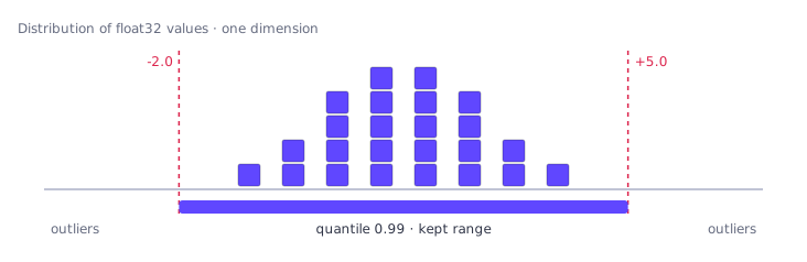
Our example shows that 99% of the values come from a [-2.0, 5.0] range. And the
conversion to int8 will surely lose some precision, so we rather prefer keeping the
representation accuracy within the range of 99% of the most probable values and ignoring
the precision of the outliers. There might be a different choice of the range width,
actually, any value from a range [0, 1], where 0 means empty range, and 1 would
keep all the values. That’s a hyperparameter of the procedure called quantile. A value
of 0.95 or 0.99 is typically a reasonable choice, but in general quantile ∈ [0, 1].
Conversion to Integers
Let’s talk about the conversion to int8. Integers also have a finite set of values that
might be represented. Within a single byte they may represent up to 256 different values,
either from [-128, 127] or [0, 255].

Since we put some boundaries on the numbers that might be represented by the f32, and
i8 has some natural boundaries, the process of converting the values between those
two ranges is quite natural:
$$ f32 = \alpha \times i8 + offset $$
$$ i8 = \frac{f32 - offset}{\alpha} $$
The parameters $ \alpha $ and $ offset $ have to be calculated for a given set of vectors,
but that comes easily by putting the minimum and maximum of the represented range for
both f32 and i8.
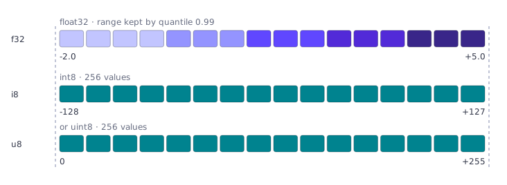
For the unsigned int8 it will go as following:
$$ \begin{equation} \begin{cases} -2 = \alpha \times 0 + offset \\ 5 = \alpha \times 255 + offset \end{cases} \end{equation} $$
In case of signed int8, we’ll just change the represented range boundaries:
$$ \begin{equation} \begin{cases} -2 = \alpha \times (-128) + offset \\ 5 = \alpha \times 127 + offset \end{cases} \end{equation} $$
For any set of vector values we can simply calculate the $ \alpha $ and $ offset $ and those values have to be stored along with the collection to enable the conversion between the types.
Distance Calculation
We do not store the vectors in the collections represented by int8 instead of float32
just for the sake of compressing the memory. But the coordinates are being used while we
calculate the distance between the vectors. Both dot product and cosine distance require
multiplying the corresponding coordinates of two vectors, so that’s the operation we
perform quite often on float32. Here is how it would look like if we perform the
conversion to int8:
$$ f32 \times f32’ = $$ $$ = (\alpha \times i8 + offset) \times (\alpha \times i8’ + offset) = $$ $$ = \alpha^{2} \times i8 \times i8’ + \underbrace{offset \times \alpha \times i8’ + offset \times \alpha \times i8 + offset^{2}}_\text{pre-compute} $$
The first term, $ \alpha^{2} \times i8 \times i8’ $ has to be calculated when we measure the distance as it depends on both vectors. However, both the second and the third term ($ offset \times \alpha \times i8’ $ and $ offset \times \alpha \times i8 $ respectively), depend only on a single vector and those might be precomputed and kept for each vector. The last term, $ offset^{2} $ does not depend on any of the values, so it might be even computed once and reused.
If we had to calculate all the terms to measure the distance, the performance could have been even worse than without the conversion. But thanks for the fact we can precompute the majority of the terms, things are getting simpler. And it turns out the scalar quantization has a positive impact not only on the memory usage, but also on the performance. As usual, we performed some benchmarks to support this statement!
Benchmarks
These benchmarks were run in March 2023 on Qdrant v1.1.0, the release that introduced scalar quantization. The hardware was not recorded, so read them as a historical comparison, not as current performance.
We simply used the same approach as we use in all the other benchmarks we publish. Both Arxiv-titles-384-angular-no-filters and Gist-960 datasets were chosen to make the comparison between non-quantized and quantized vectors. The results are summarized in the tables:
Arxiv-titles-384-angular-no-filters
| Upload and indexing time | Mean search precision, ef = 128 | Mean search time, ef = 128 | Mean search precision, ef = 256 | Mean search time, ef = 256 | Mean search precision, ef = 512 | Mean search time, ef = 512 | |
|---|---|---|---|---|---|---|---|
| Non-quantized vectors | 649 s | 0.989 | 0.0094 | 0.994 | 0.0932 | 0.996 | 0.161 |
| Scalar Quantization | 496 s | 0.986 | 0.0037 | 0.993 | 0.060 | 0.996 | 0.115 |
| Difference | -23.57% | -0.3% | -60.64% | -0.1% | -35.62% | 0% | -28.57% |
A slight decrease in search precision results in a considerable improvement in the latency. Unless you aim for the highest precision possible, you should not notice the difference in your search quality.
Gist-960
| Upload and indexing time | Mean search precision, ef = 128 | Mean search time, ef = 128 | Mean search precision, ef = 256 | Mean search time, ef = 256 | Mean search precision, ef = 512 | Mean search time, ef = 512 | |
|---|---|---|---|---|---|---|---|
| Non-quantized vectors | 452 s | 0.802 | 0.077 | 0.887 | 0.135 | 0.941 | 0.231 |
| Scalar Quantization | 312 s | 0.802 | 0.043 | 0.888 | 0.077 | 0.941 | 0.135 |
| Difference | -30.97% | 0% | -44.16% | +0.11% | -42.96% | 0% | -41.56% |
In all the cases, the decrease in search precision is negligible, but we keep a latency reduction of at least 28.57%, even up to 60.64%, while searching. As a rule of thumb, the higher the dimensionality of the vectors, the lower the precision loss.
Oversampling and Rescoring
A distinctive feature of the Qdrant architecture is the ability to combine the search for quantized and original vectors in a single query. This enables the best combination of speed, accuracy, and RAM usage.
Qdrant stores the original vectors, so it is possible to rescore the top-k results with the original vectors after doing the neighbours search in quantized space. That obviously has some impact on the performance, but in order to measure how big it is, we made the comparison in different search scenarios. We used a machine with a very slow network-mounted disk and tested the following scenarios with different amounts of allowed RAM:
| Setup | RPS | Precision |
|---|---|---|
| 4.5GB memory | 600 | 0.99 |
| 4.5GB memory + SQ + rescore | 1000 | 0.989 |
And another group with more strict memory limits:
| Setup | RPS | Precision |
|---|---|---|
| 2GB memory | 2 | 0.99 |
| 2GB memory + SQ + rescore | 30 | 0.989 |
| 2GB memory + SQ + no rescore | 1200 | 0.974 |
In those experiments, throughput was mainly defined by the number of disk reads, and quantization efficiently reduces it by allowing more vectors in RAM. Read more about on-disk storage in Qdrant and how we measure its performance in our article: Minimal RAM you need to serve a million vectors .
The mechanism of Scalar Quantization with rescoring disabled pushes the limits of low-end machines even further. It seems like handling lots of requests does not require an expensive setup if you can agree to a small decrease in the search precision.
Where Scalar Quantization Fits Today
Qdrant offers more quantization methods today than it did in 2023. Scalar quantization is still what the documentation recommends at 4x compression. Since v1.18, 4-bit TurboQuant gives comparable recall at 8x compression, unless you use the Manhattan (L1) distance. Binary quantization and product quantization go further, up to 32x and 64x, at a larger accuracy cost. The quantization guide compares the methods by compression level.
To see how scalar quantization compares with 4-bit TurboQuant today, we reran Gist-960 in October 2026 on Qdrant v1.19.2. Every run used the same collection: HNSW with m=16 and ef_construct=100, Euclidean distance, original vectors on disk, and quantized vectors in RAM. Recall@10 is measured against the dataset’s ground-truth neighbors, and rescoring uses no oversampling.
| Method | Compression | Recall@10, ef=128 | Recall@10, ef=256 | Recall@10, ef=512 |
|---|---|---|---|---|
| No quantization | 1x | 0.928 | 0.962 | 0.981 |
| Scalar quantization, rescore | 4x | 0.929 | 0.964 | 0.983 |
| Scalar quantization, no rescore | 4x | 0.887 | 0.914 | 0.927 |
| 4-bit TurboQuant, rescore | 8x | 0.929 | 0.965 | 0.981 |
| 4-bit TurboQuant, no rescore | 8x | 0.878 | 0.903 | 0.912 |
With rescoring, scalar quantization and 4-bit TurboQuant both land within 0.003 of the unquantized baseline, and TurboQuant uses half the memory of scalar quantization. Those gaps are smaller than the variation between HNSW builds: an earlier run on Qdrant v1.19.1 moved individual results by up to 0.008. Without rescoring, scalar quantization kept 0.009 to 0.016 more recall than TurboQuant in both runs. The runs measured recall only, not latency. The 2023 settings were not recorded, so compare rows within this table rather than with the 2023 tables.
Accessing Best Practices
Qdrant documentation on Scalar Quantization is a great resource describing different scenarios and strategies to achieve up to 4x lower memory footprint and even up to 2x performance increase.
Further Reading
- Quantization guide: how to configure each method, and which one to choose at each compression level.
- TurboQuant in Qdrant: the 8x method compared with scalar quantization in this article.
- Binary Quantization and Product Quantization: the options for higher compression.
- Minimal RAM to serve a million vectors: how on-disk storage and quantization reduce memory use.
- Gist-960 on ann-benchmarks: the dataset and ground-truth neighbors used for the 2026 rerun.
- Reproduction kit: the script and raw results to rerun the 2026 table on your Qdrant version.