Module 1

Late Interaction Basics

When building a search system, one fundamental question emerges: when should a query and document interact? The answer to this question may affect both the quality of search results and the system’s scalability.

This lesson introduces the late interaction paradigm - the foundation of multi-vector search - and explores how it compares to other approaches.

Follow along in Colab:

Understanding the Alternatives

Before diving into late interaction, let’s establish what we mean by “interaction.”

In search systems, interaction refers to when and how the query and document representations influence each other. Do they interact during encoding, or only during comparison? This timing fundamentally shapes the system’s architecture.

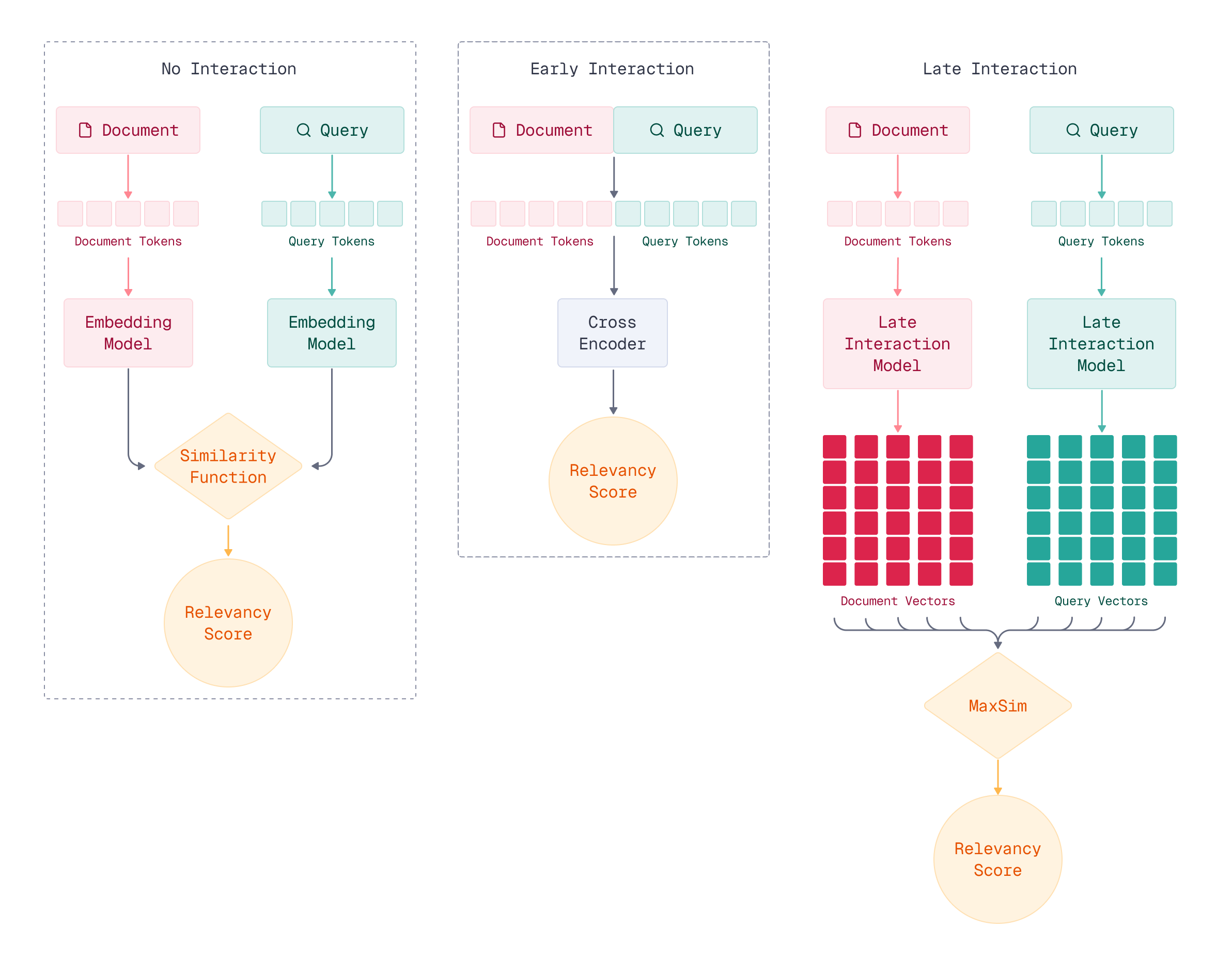
We can categorize approaches based on when this interaction occurs:

• No interaction: Query and document are encoded independently into fixed representations, then compared. They never “see” each other during encoding.
• Early interaction: Query and document are encoded together, with each word attending to the other during the encoding process. Maximum interaction, but no pre-computation.
• Late interaction: Query and document are encoded independently (like no interaction), but we preserve fine-grained representations that interact during scoring (late in the process).

Let’s examine each paradigm to understand the trade-offs. A simple example will illustrate the differences between all the methods.

# Example documents and query we'll use throughout this lesson
documents = [
    "Qdrant is an AI-native vector database and a semantic search engine",
    "Relational databases are not well-suited for search",
]
query = "What is Qdrant?"

Single-Vector Embeddings (No Interaction)

The most common approach encodes each document and query into a single dense vector, then compares them using similarity (most often cosine similarity).

The strength: This method is simple, fast, and scales well. Document vectors can be pre-computed and stored, making search efficient even across billions of documents.

The limitation: Compressing an entire document into a single vector means losing fine-grained details. Think of it like summarizing a book in one sentence - you capture the general theme but miss the nuances that might be relevant to a specific query.

Let’s load a dense embedding model and generate vector representations for our documents.

from fastembed import TextEmbedding

# Load the BAAI/bge-small-en-v1.5 model
dense_model = TextEmbedding("BAAI/bge-small-en-v1.5")
# Pass the documents through the model. The .passage_embed
# method returns a generator we can iterate over and is
# supposed to be used for the documents only.
dense_generator = dense_model.passage_embed(documents)
# Running next on the generator yields one vector at
# the time, representing a single document.
dense_vector = next(dense_generator)

We also need to generate a vector for the query using the same model.

# Generate a dense vector for the query as well, using
# the .query_embed method this time.
dense_query_vector = next(dense_model.query_embed(query))

Now we can calculate the similarity between the query and each document using the dot product.

import numpy as np

# Calculate the dot product between the query
# and the first document vector
np.dot(dense_query_vector, dense_vector)

Let’s calculate the similarity with the second document as well.

# Calculate the dot product between the same query
# and the second document vectors
np.dot(dense_query_vector, next(dense_generator))

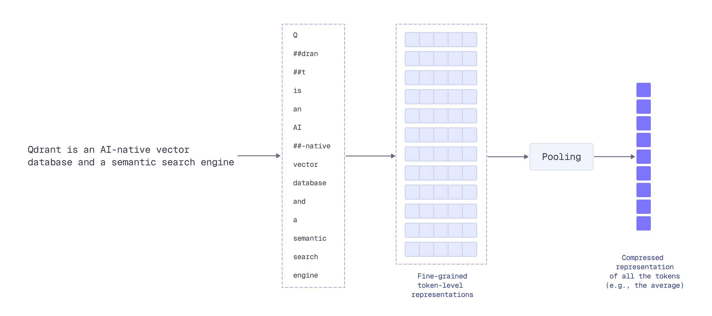
Notice how each document and query produces exactly one vector of 384 dimensions. To achieve this compression, the model internally generates embeddings for each token, then uses pooling (typically mean pooling or a special [CLS] token) to aggregate them into a single fixed-size representation.

Cross-Encoders (Early Interaction)

At the other extreme, cross-encoders process the query and document together through a neural network, producing a relevance score. This is “early interaction” because the query and document interact during the encoding phase itself.

The strength: This approach achieves deep contextual understanding. Every query word can “attend to” every document word during encoding, enabling precise relevance judgments.

The limitation: You must process every query-document pair from scratch. For a collection of a million documents, that means a million forward passes through a neural network for each query - prohibitively expensive for initial retrieval.

Cross-encoders excel at re-ranking a small candidate set but don’t scale for searching large collections.

Let’s see how cross-encoders work differently by processing the query and documents together.

from fastembed.rerank.cross_encoder import TextCrossEncoder

# Load the Xenova/ms-marco-MiniLM-L-6-v2 cross encoder model
cross_encoder = TextCrossEncoder("Xenova/ms-marco-MiniLM-L-6-v2")
# Run .rerank method on the query and all the documents.
# It does not create any vector representations, but gives
# the score indicating the relevance of the document for
# the provided query.
cross_encoder.rerank(query, documents)

The key difference: cross-encoders cannot pre-compute document representations. Each query requires fresh computation for every candidate, making them impractical for initial retrieval over large collections.

The Gap

We need an approach that combines the best of both worlds: the scalability of pre-computed single-vector representations and the fine-grained matching capability of cross-encoders.

Late Interaction: The Core Paradigm

Late interaction solves this challenge through a simple but powerful idea: encode documents and queries into multiple token-level vectors, then defer the comparison until search time.

How It Works

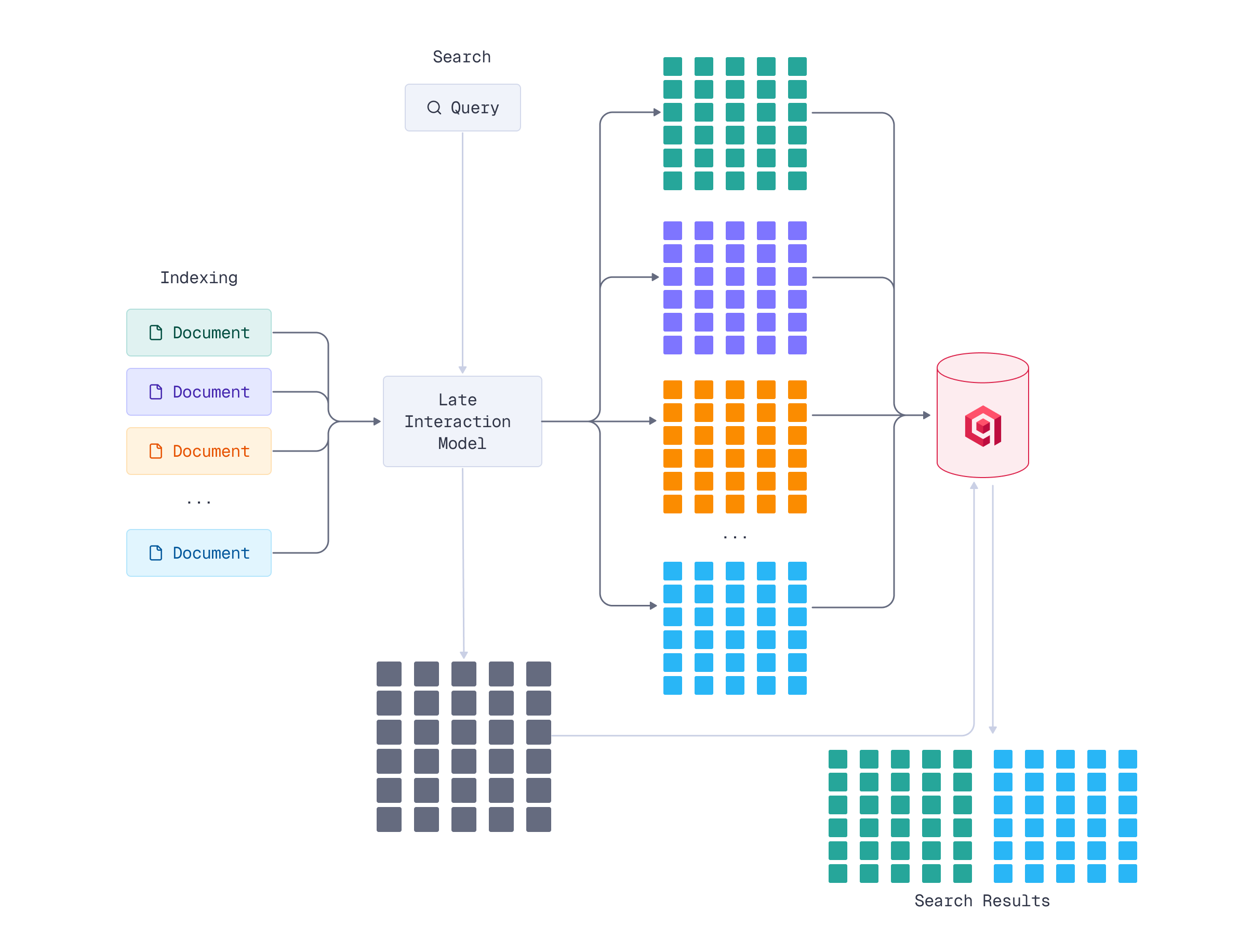
Instead of compressing a document into a single vector, late interaction represents it as a collection of contextualized token embeddings

1. Encode: Pass the document through an encoder (like ColBERT) to generate one embedding vector per token
2. Store multi-vector representations: Keep all token vectors instead of aggregating them into a single vector
3. Defer comparison: At search time, compare query token vectors against document token vectors
4. Late interaction: The actual “interaction” between query and document happens late - only when computing relevance scores

This isn’t that much fundamentally different from both single-vector and cross-encoder approaches, yet there are some differences:

• Unlike single-vector: We preserve fine-grained, token-level information
• Unlike cross-encoders: We encode documents independently, enabling pre-computation

Key Benefits

Pre-computation: Document embeddings can be computed once and stored, just like single-vector approaches. You don’t need to re-encode documents for every query.

Fine-grained matching: Different query terms can match different parts of the document. A query about “apple computer” can distinguish contextual meaning from “apple fruit” based on which document tokens match strongly.

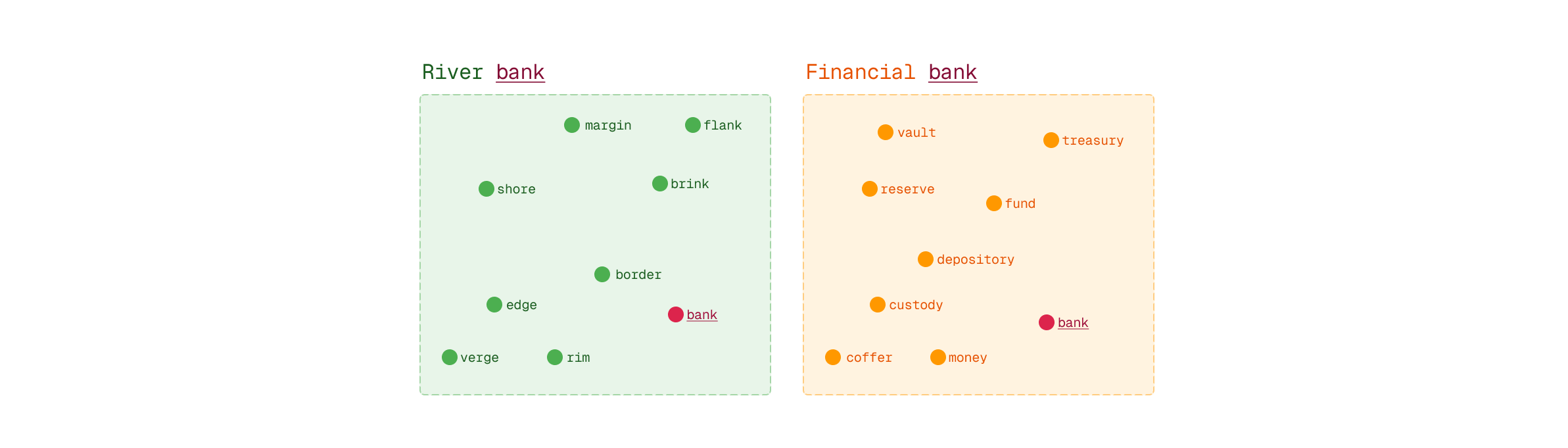
Contextual understanding: Token embeddings are contextualized by the surrounding text. The word “bank” has different embeddings in “river bank” versus “financial bank.”

Scalability: While requiring more storage than single vectors, the deferred comparison enables searching large collections efficiently.

The ColBERT Approach

The canonical implementation of late interaction is ColBERT (Contextualized Late Interaction over BERT), developed at Stanford. ColBERT popularized this paradigm and demonstrated that you can achieve cross-encoder-level effectiveness with single-vector-level efficiency.

The core innovation: maintaining bags of contextualized embeddings and delaying the interaction computation until the final stage.

Let’s load a ColBERT model and generate multi-vector representations for our documents.

from fastembed import LateInteractionTextEmbedding

# Load the colbert-ir/colbertv2.0 model
colbert_model = LateInteractionTextEmbedding("colbert-ir/colbertv2.0")
# Run .passage_embed on all the documents and create
# a generator of the multi-vector representations
colbert_generator = colbert_model.passage_embed(documents)
colbert_vector = next(colbert_generator)

Similarly, we create a multi-vector representation for the query.

# Create multi-vector representation for the query
colbert_query_vector = next(colbert_model.query_embed(query))

Key observation: Unlike single-vector search, each document is represented by multiple vectors. At search time, we compare each query token against all document tokens to compute a relevance score.

Why This Matters for Multi-Vector Search

Late interaction isn’t just a technical optimization - it represents a fundamental shift in how we think about semantic search.

Captures semantic nuance: Because we maintain multiple vectors per document, the system can capture complex, multi-faceted content. A document about “Python programming for data science” can match queries about programming languages, data analysis, and scientific computing - each matching different token sets.

Enables scale: Pre-computed multi-vector representations mean you can build practical search systems over large document collections. The computational cost grows with collection size, not quadratically with query-document pairs.

Foundation for this course: Everything we’ll explore in subsequent lessons builds on this paradigm - from the distance metrics that enable multi-vector comparison to multi-modal extensions like ColPali to optimization techniques for production deployment.

Beyond text: The late interaction paradigm extends naturally to other modalities. Module 2 explores how ColPali applies these same principles to visual documents, enabling semantic search over images and PDFs.

What’s Next

Understanding the conceptual foundation of late interaction is the first step. But how exactly do we compare sets of query vectors against sets of document vectors?

In the next lesson, you’ll learn about MaxSim - the distance metric that powers late interaction search. MaxSim defines the specific mathematical operation for computing similarity between multi-vector representations.

From there, we’ll explore use cases where multi-vector search excels, challenges you’ll face in production, and how to implement these techniques in Qdrant.