Module 1

MaxSim Distance Metric

MaxSim (Maximum Similarity) is the core distance metric for late interaction models. Unlike traditional vector similarity metrics that operate on pairs of single vectors, MaxSim computes similarity between sequences of vectors.

Understanding MaxSim is important for working with multi-vector search effectively and understanding its performance characteristics.

Follow along in Colab:

The MaxSim Formula

In late interaction, we represent documents and queries as sequences of token vectors. But how do we measure similarity between two sets of vectors?

The answer is MaxSim (Maximum Similarity), defined mathematically as:

$MaxSim (Q, D) = \sum_{i = 1}^{| Q |} {max}_{j = 1}^{| D |} sim (q_{i}, d_{j})$

Where:

$Q$ represents the query token vectors
$D$ represents the document token vectors
$sim (q_{i}, d_{j})$ is a base similarity function that measures the distance between two vectors

The $sim (q_{i}, d_{j})$ function can be any distance metric - dot product, cosine similarity, Euclidean distance, or others. Let’s break down what this formula actually computes.

Understanding MaxSim Step-by-Step

The Computation Process

Let’s make this concrete with an example. Consider:

Query: “apple computer”
Document: “Apple makes the MacBook laptop”

MaxSim formula will choose the strongest connection from the query tokens to document tokens and sum the strengths of each connection for all the query tokens.

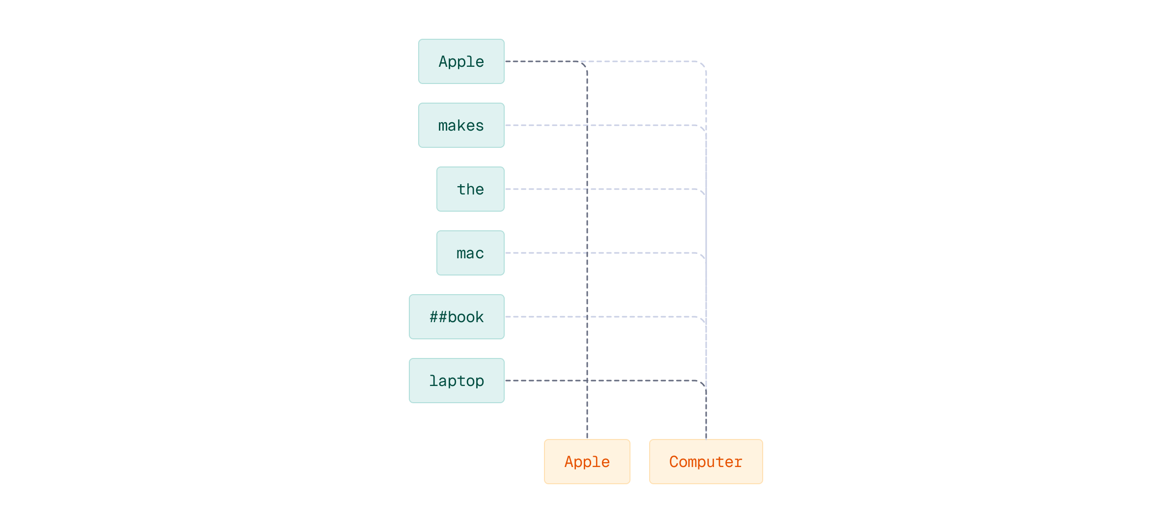
The key insight here: each query token finds its best match in the document. This enables fine-grained semantic matching - instead of comparing holistic document representations, we’re allowing each part of the query to independently find its most relevant counterpart.

Let’s walk through this with a concrete example:

query = "apple computer"
document = "Apple makes the MacBook laptop"

Next, we load the ColBERT model to generate multi-vector representations for both the query and document:

from fastembed import LateInteractionTextEmbedding

# Load the colbert-ir/colbertv2.0 model
colbert_model = LateInteractionTextEmbedding("colbert-ir/colbertv2.0")

# Create multi-vector representations of the query and document
query_vector = next(colbert_model.query_embed(query))
document_vector = next(colbert_model.passage_embed(document))

Understanding Tokenization

Before we compute MaxSim, let’s understand how ColBERT tokenizes our query and document. This tokenization is crucial because each token gets its own embedding vector.

query_tokenization = colbert_model.model.tokenize([query])[0]
query_tokenization.tokens

This shows how the query tokenizes into individual tokens including special tokens like [CLS] and [SEP].

document_tokenization = colbert_model.model.tokenize([document])[0]
document_tokenization.tokens

Similarly, the document is tokenized. Notice that words like ‘MacBook’ may be split into subword tokens using WordPiece tokenization (e.g., ‘mac’ and ‘##book’). Each token will get its own embedding vector.

Now let’s compute MaxSim step-by-step. For each query token, we’ll find its maximum similarity score across all document tokens, then sum these maxima:

import numpy as np

similarity = 0.0
for qt, qt_vector in zip(query_tokenization.tokens,
                         query_vector):
    max_idx, max_sim = 0, np.dot(qt_vector, document_vector[0])
    for i, dt_vector in enumerate(document_vector[1:], start=1):
        distance = np.dot(qt_vector, dt_vector)
        if distance > max_sim:
            max_idx, max_sim = i, distance

    print(qt, max_idx, max_sim)
    similarity += max_sim

The code iterates through each query token, computes its dot product similarity with every document token, and keeps track of the maximum. The print statement shows which document position each query token matched best with and the similarity score. Each query token independently seeks its strongest counterpart in the document.

print("MaxSim(Q, D) =", similarity)

The final MaxSim(Q, D) score is the sum of all these maximum similarities.

The Intuition Behind MaxSim

MaxSim implements token-level relevance matching. Each query term actively seeks its most relevant counterpart in the document. Unlike single-vector search where you compare one query vector to one document vector (one-to-one), MaxSim performs many-to-many matching. This enables contextual precision. When you search for “apple computer”, the word “apple” in your query will match strongly with “Apple” (the company name) in documents about technology, not “apple” (the fruit) in documents about nutrition, as contextualized token embeddings should capture these semantic distinctions.

But why maximum and not average? Consider a query about “Python programming”. A document might discuss Python extensively in one section but also mention cooking recipes in another. MaxSim focuses on the strong matches (Python-related tokens) rather than diluting the score with irrelevant tokens. This design choice reflects a fundamental insight: relevance is often concentrated, not uniform.

The HNSW Challenge

There’s a significant challenge related to MaxSim when it comes to indexing these representations efficiently. HNSW (Hierarchical Navigable Small World) graphs enable fast approximate nearest neighbor search by building static proximity graphs. They rely on the assumption that distance functions must be symmetric and query-independent. This allows HNSW to construct fixed neighbor relationships that makes the effective graph traversal possible.

MaxSim breaks this assumption by design. Looking back at the formula, notice that $Q$ and $D$ play fundamentally different roles:

We iterate over query tokens - each query token contributes to the final sum
Documents are what we search within - we take the maximum similarity from document tokens for each query token

This non-symmetrical structure means MaxSim(Q, D) ≠ MaxSim(D, Q). When you swap the parameters, you change which tokens contribute to the sum.

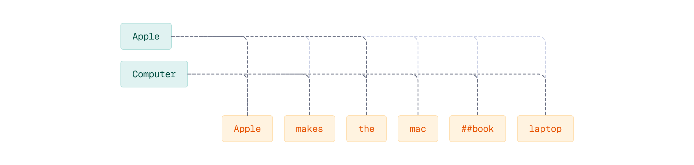
To illustrate this asymmetry concretely, let’s compute MaxSim in reverse - iterating over document tokens instead of query tokens:

similarity = 0.0
for dt, dt_vector in zip(document_tokenization.tokens,
                         document_vector):
    max_idx, max_sim = 0, np.dot(dt_vector, query_vector[0])
    for i, qt_vector in enumerate(query_vector[1:], start=1):
        distance = np.dot(dt_vector, qt_vector)
        if distance > max_sim:
            max_idx, max_sim = i, distance

    print(dt, max_idx, max_sim)
    similarity += max_sim

Now the iteration is different: we loop over document tokens instead of query tokens. Since the document has more tokens than the query, we’re summing over more terms, which fundamentally changes the computation.

print("MaxSim(D, Q) =", similarity)

The MaxSim(D, Q) score will be different from MaxSim(Q, D) because we iterated over a different number of tokens. This asymmetry occurs because:

We summed over document tokens instead of query tokens (different number of terms)
The iteration direction changed the fundamental computation
Query and document play fundamentally different roles in the formula

This non-symmetry is why HNSW indexing becomes problematic for MaxSim - nearest neighbor relationships change depending on which direction you query.

A document’s nearest neighbors are query-dependent and change based on which query you’re processing, making it impossible to build the static proximity graph that HNSW requires. The practical reality is you must compute MaxSim against every document at query time with brute force comparison. For large collections, this becomes slow, or even impossible.

The common solution is two-stage retrieval, and we’ll explore that pattern in later lessons and see how Qdrant optimizes multi-vector search.

Connecting the Concepts

In the previous lesson, you learned about the late interaction paradigm - encoding queries and documents into multiple token vectors and deferring comparison until search time. MaxSim is the mathematical operation that makes this deferred comparison work. It’s the bridge between the conceptual model (multi-vector representations) and practical implementation. Without MaxSim or a similar aggregation function, we’d have no way to score documents against queries when both are represented as sequences of vectors.

What’s Next

MaxSim gives us a way to compare multi-vector representations, capturing fine-grained semantic matching that single-vector search cannot achieve. But as we’ve seen, it also introduces significant computational challenges - particularly the asymmetry that breaks traditional indexing approaches like HNSW.

In the next lesson, we’ll explore use cases where multi-vector search excels despite these challenges. You’ll see scenarios where the improved relevance and semantic precision justify the additional computational cost.

From there, we’ll learn how to implement efficient multi-vector search in Qdrant, including the hybrid retrieval patterns that make late interaction practical at scale.

Continue to Next Step

MaxSim Distance Metric

The MaxSim Formula

Understanding MaxSim Step-by-Step

The Computation Process

Understanding Tokenization

The Intuition Behind MaxSim

The HNSW Challenge

Connecting the Concepts

What’s Next

About cookies on this site

Targeting Cookies

Functional Cookies

Strictly Necessary Cookies

Performance Cookies