Module 2

How ColPali Models Work

ColPali extends the late interaction paradigm from text to visual documents. It can process PDFs, images, and scanned documents, generating multi-vector representations that capture both textual and visual information.

Understanding ColPali’s architecture helps you leverage its full potential for multi-modal document retrieval.

Follow along in Colab:

From Text to Visual Documents

What about documents that aren’t just text? PDFs often contain diagrams, tables, charts, equations, and complex layouts where the visual presentation carries as much meaning as the text itself.

Traditional approaches to searching visual documents typically involve two steps: first, extract text using OCR (Optical Character Recognition), then search the extracted text. This pipeline has significant limitations:

• Lost layout information: OCR converts documents to plain text, discarding spatial relationships and visual structure
• Diagram blindness: Charts, graphs, and diagrams are either ignored or poorly represented
• Format fragility: Tables, mathematical notation, and multi-column layouts often get mangled during text extraction

ColPali takes a fundamentally different approach: it treats the document image itself as the primary representation. ColPali “tokenizes” images into spatial patches. Each patch becomes a visual token with its own embedding, enabling token-level matching without ever extracting text.

This means ColPali can match queries directly to visual regions of document pages - no OCR required.

The Vision Language Model Foundation

Before diving into how ColPali processes images, let’s understand its architectural foundation. ColPali isn’t built from scratch - it’s based on sophisticated Vision Language Models (VLMs) that already understand the relationship between visual and textual information.

Building on PaliGemma

ColPali v1.3 is built on PaliGemma-3B, a Vision Language Model that combines two powerful components:

• SigLIP-So400m (Vision Encoder): Processes images into visual features
• Gemma-2B (Language Model): Contextualizes those features using transformer layers

Why use a VLM instead of training a vision model from scratch? VLMs are pre-trained on massive datasets of image-text pairs, so they already “understand” how visual content relates to language. This makes them ideal for document retrieval: they can naturally connect text queries to corresponding visual content.

PaliGemma was specifically designed for tasks requiring both visual understanding and language processing - perfect for searching documents that blend text, diagrams, tables, and equations.

Fine-tuning for Document Retrieval: The base PaliGemma model is adapted for document retrieval using LoRA (Low-Rank Adaptation), a parameter-efficient technique that specializes the model without retraining everything. The vision encoder stays frozen while attention layers are fine-tuned to optimize for document search.

The Two-Component Architecture

Think of ColPali’s architecture as having “eyes” and a “brain”:

Vision Encoder (SigLIP) - The Eyes:

• Takes the document image and divides it into patches (the 32×32 grid we’ll explore next)
• Processes each patch through a vision transformer
• Outputs visual features that capture what’s in each patch: text characters, diagram elements, table cells, etc.

Language Model (Gemma-2B) - The Brain:

• Receives the visual features from SigLIP
• Runs them through transformer layers to add context and semantic understanding
• Each patch’s features get enriched by understanding neighboring patches
• Outputs contextualized representations that understand relationships across the document

The Flow: Image patches are first processed through the SigLIP encoder to generate visual features. These visual features then pass through the Gemma-2B transformer, which produces contextualized representations. Finally, the contextualized representations flow through a projection layer to produce 128-dimensional embeddings. This pipeline ensures that each 128-dim embedding doesn’t just capture what’s in one patch - it understands that patch in the context of the entire document.

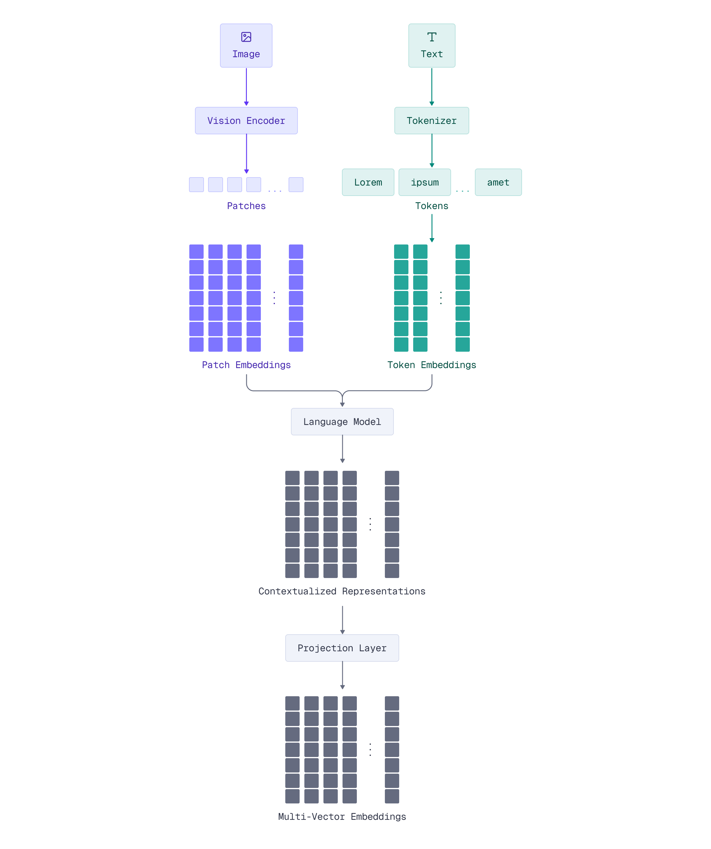
For text inputs, there isn’t any additional preprocessing step, but it is tokenized and passed through the language model. This architecture can use the same “brain” to process different modalities.

Patch-Based Image Processing

Vision transformers, the foundation of ColPali, don’t process entire images at once. Instead, they divide images into a grid of fixed-size patches - think of it like a checkerboard overlaid on your document.

The ColPali pipeline starts with a document. It is usually a screenshot of a single PDF page, or anything you want to encode. While you might convert a PDF page to a high-resolution screenshot to preserve visual details during conversion, the ColPali preprocessing itself resizes images to a fixed resolution of 448×448 pixels before processing.

This fixed-size input is then divided into patches:

• Patch size: 14×14 pixels per patch
• Patch grid: 32×32 patches (448 / 14 = 32 patches per side)
• Total patches: 1024 patches per image (32 × 32 = 1024)

Each patch becomes a visual “token” representing a spatial region of the document. A patch might contain part of a diagram, a few words of text, a piece of an equation, or even just whitespace - each gets its own embedding. This consistent structure ensures predictable embedding sizes and simplifies the search pipeline.

Token Structure and Embeddings

Now that you understand ColPali’s VLM foundation - SigLIP processing patches, Gemma-2B contextualizing features, and the projection layer generating embeddings - let’s see how this architecture processes images into the final multi-vector representation.

When ColPali processes an image, the PaliGemma model doesn’t just generate patch embeddings directly. It creates a sequence of tokens that flows through the entire architecture we just described. This sequence includes both the image patches and additional instruction tokens that help guide the model’s behavior.

For a single document image, the token sequence contains:

• 1024 special <image> tokens - one for each patch in the 32×32 grid
• Instruction tokens - additional tokens that help the model understand its task

<image><image>...<image><bos>Describe the image.\n

The final embedding output contains 1030 vectors of 128 dimensions each: 1024 for the image patches plus 6 additional instruction tokens. For search purposes, all vectors participate in the MaxSim calculation - each query token finds its best match among all 1030 vectors.

With this multi-vector representation, each query word finds its best match among all 1030 visual vectors using late interaction. Query terms match to the most semantically similar patches - whether those patches contain diagrams, text, tables, or equations - exactly the same MaxSim scoring we learned about in Module 1, but extended to visual documents.

Implementing Multi-Modal Search with FastEmbed and Qdrant

Now that you understand ColPali’s architecture - from its VLM foundation to patch-based processing to multi-vector embeddings - let’s build a practical multi-modal search system. We’ll again use FastEmbed, as it also provides a unified interface for multi-modal late interaction models like ColPali.

Loading ColPali with FastEmbed

Let’s start by loading a ColPali model. FastEmbed supports several ColPali variants, but in this lesson we’ll use ColPali v1.3:

from fastembed import LateInteractionMultimodalEmbedding

# Load the Qdrant/colpali-v1.3-fp16 model from HF hub
colpali_model = LateInteractionMultimodalEmbedding(
    model_name="Qdrant/colpali-v1.3-fp16"
)

This single initialization loads the entire ColPali architecture we discussed: SigLIP vision encoder, Gemma-2B language model, and the projection layer. The LateInteractionMultimodalEmbedding class handles both image and text encoding through a unified interface, encapsulating the image and text processing logic so you can just pass image paths or queries.

Processing Images and Understanding Embeddings

Now let’s process a document image through ColPali to see the multi-vector embeddings in action:

from PIL import Image

image = Image.open("images/einstein-newspaper.jpg")
image

Now let’s generate the embeddings:

# Create the representation of the image
colpali_generator = colpali_model.embed_image(["images/einstein-newspaper.jpg"])
document_vectors = next(colpali_generator)
document_vectors.shape

The output shape shows 1030 vectors of 128 dimensions each. These 1030 vectors include the 1024 image patch embeddings (from the 32×32 grid) plus 6 additional instruction tokens used by the model.

Processing query text:

ColPali also encodes text queries into multi-vector representations:

# Create the representation of the query
query = "When did dr. Einstein die?"
query_vectors = next(colpali_model.embed_text(query))
query_vectors.shape

Let’s define a helper function to compute the MaxSim score:

import numpy as np

def maxsim(Q, D):
    sims = np.dot(Q, D.T)
    max_sims = sims.max(axis=1)
    return max_sims.sum()

Now finally compute the score:

maxsim(query_vectors, document_vectors)

During search, each query token finds its best match among all 1030 document vectors using MaxSim - the same late interaction scoring we learned in Module 1. A higher score indicates better semantic overlap between the query and the visual document.

Setting Up Qdrant for Multi-Vector Search

To store and search these multi-vector embeddings, we need a Qdrant collection configured for late interaction:

from qdrant_client import QdrantClient, models

client = QdrantClient("http://localhost:6333")

client.create_collection(
    collection_name="colpali",
    vectors_config={
        "colpali-v1.3": models.VectorParams(
            size=128,
            distance=models.Distance.DOT,
            multivector_config=models.MultiVectorConfig(
                comparator=models.MultiVectorComparator.MAX_SIM,
            ),
            hnsw_config=models.HnswConfigDiff(m=0),
        ),
    },
)

This configuration mirrors what you learned in Module 1 - multi-vector config with MAX_SIM comparator, dot product distance, and HNSW disabled.

Indexing Visual Documents

Now let’s index visual documents using Qdrant’s local inference feature. This approach uses models.Image() to let Qdrant handle embedding generation automatically via FastEmbed:

import uuid

documents = [
    "images/einstein-newspaper.jpg",
    "images/titanic-newspaper.jpg",
    "images/men-walk-on-moon-newspaper.jpg",
]
client.upsert(
    collection_name="colpali",
    points=[
        models.PointStruct(
            id=uuid.uuid4().hex,
            vector={
                "colpali-v1.3": models.Image(
                    image=doc,
                    model="Qdrant/colpali-v1.3-fp16",
                )
            },
            payload={
                "image": doc,
            }
        )
        for doc in documents
    ]
)

This uses local inference - similar to models.Document() for text that you saw in Module 1. Qdrant’s FastEmbed integration processes images locally (not on a remote server), generating the multi-vector embeddings automatically. This is much simpler than manually generating embeddings with FastEmbed and then upserting them.

Once indexed, each document image is represented by its 1030 vectors (1024 patches + 6 instruction tokens), ready for late interaction search. When a query comes in, Qdrant will compute MaxSim scores between the query tokens and these vectors.

Querying with Late Interaction

The power of ColPali becomes clear when searching. Using local inference, you can query with text and match against visual documents:

client.query_points(
    collection_name="colpali",
    query=models.Document(
        text="Who was the first man on the moon?",
        model="Qdrant/colpali-v1.3-fp16",
    ),
    using="colpali-v1.3",
    limit=2,
)

This uses the same local inference pattern you saw in Module 1 with models.Document(). Qdrant handles query tokenization, embedding generation, and MaxSim computation automatically.

Let’s try different queries:

client.query_points(
    collection_name="colpali",
    query=models.Document(
        text="Why did Titanic sink?",
        model="Qdrant/colpali-v1.3-fp16",
    ),
    using="colpali-v1.3",
    limit=2,
)

How late interaction works for visual search:

1. Your query is tokenized into query embeddings (e.g., 6-8 tokens for “Who was the first man on the moon?”)
2. For each query token, Qdrant finds the maximum similarity across all 1030 visual vectors of each document image
3. The maximum similarities are summed (MaxSim) to score each image
4. Images with content matching the query score highest

This is text-to-image search without OCR. You’re matching the semantic meaning of text queries directly to visual content - headlines, photos, captions, and text in its original layout. The late interaction paradigm enables fine-grained matching at the token level, just like ColBERT for text, but extended to visual documents.

What’s Next

Now that you understand how ColPali works and can build basic multi-modal search systems, several questions naturally arise:

• Which ColPali model should you use? The ColPali family includes variants optimized for different hardware constraints and accuracy requirements.
• How can you interpret what the model is finding? Unlike black-box embeddings, ColPali offers powerful visualization capabilities to see exactly which image regions match your query terms.
• How do you optimize for production? Multi-vector search can be resource-intensive at scale - you’ll need techniques like quantization, pooling, and multi-stage retrieval.

In the next lesson, we’ll explore the ColPali family and learn when to use each model variant. Then, we’ll dive into visual interpretability to understand exactly what ColPali sees in your documents.