Pooling Techniques
While quantization reduces the size of each vector, pooling reduces the number of vectors per document. By intelligently combining token embeddings, you can achieve significant memory savings while preserving retrieval quality.
Follow along in Colab: ![]()
Pooling in Embedding Models
Pooling isn’t new to vector search - it’s fundamental to how most embedding models work. When you encode text with models like Sentence Transformers, the model first generates embeddings for each token in your input. But to create a single vector representing the entire text, the model must pool these token embeddings together.
Common pooling strategies in dense embedding models include:
- Mean pooling: Average all token embeddings into a single vector
- CLS token pooling: Use the special
[CLS]token’s embedding as the document representation - Max pooling: Take the maximum value for each dimension across all tokens
- Weighted pooling: Assign different importance to different tokens (e.g., using attention weights)
These techniques compress variable-length sequences of token embeddings into fixed-size vectors, making them compatible with traditional vector search systems.
With multi-vector representations, we face a similar but more nuanced challenge. Instead of reducing tokens to a single vector upfront, we maintain multiple vectors per document to preserve richer semantic information. However, as you learned in the previous lessons, this creates memory and performance challenges. Pooling techniques for multi-vector search let you strategically reduce the number of vectors while retaining the benefits of late interaction.
Important: Pooling is typically applied only to document embeddings, not queries. Why? Queries are usually short (a few tokens), so there’s little memory to save. More importantly, we want to preserve full query resolution - every query token should have the opportunity to find its best match among document tokens. The memory savings come from compressing the large document collection, not the ephemeral query vectors.
Pooling for Multi-Vector Representations
Image-Specific Methods
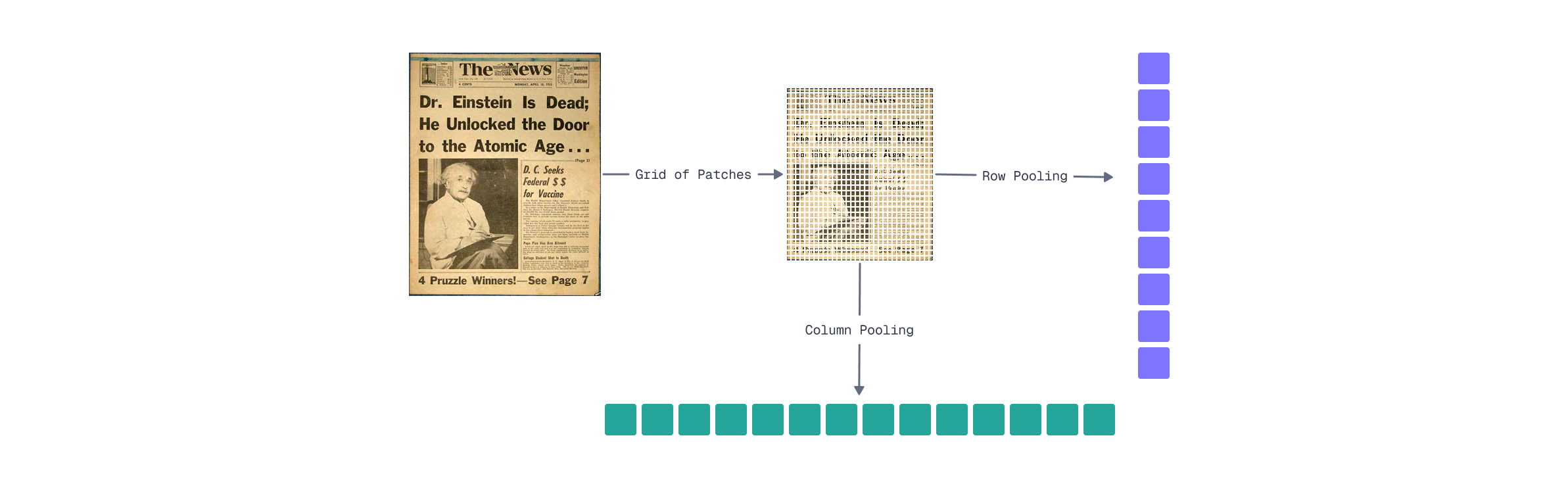
For visual document representations like ColPali, spatial relationships in the patch grid enable effective pooling strategies. As you learned in Module 2’s visual interpretability lesson, patches in the same row or column often capture semantically related content - a row might contain a line of text, while a column might capture a vertical element like a table border or sidebar.
Row pooling groups patches by their horizontal position:
- Organize the 1024 patch embeddings into a 32×32 grid
- Apply mean pooling across each row (combining 32 patches)
- Result: 32 vectors instead of 1024
Mathematically:
Where
Column pooling works similarly but along the vertical axis:
This also produces 32 vectors, but captures vertical content relationships instead.
Memory savings are substantial. FastEmbed returns embeddings in float16 format by default, which already halves the memory compared to float32:
| Representation | Vectors | Memory (float16) | Memory (float32) |
|---|---|---|---|
| Full patches | 1024 | 256 KB | 512 KB |
| Row pooling | 32 | 8 KB | 16 KB |
| Column pooling | 32 | 8 KB | 16 KB |
That’s a 32× reduction in vector count and memory footprint.
Trade-offs to consider:
- Loss of fine-grained resolution: Small details that span partial rows may blend together
- Row pooling may work better for horizontally-oriented content, like text
- Column pooling may better capture vertical structures like tables, sidebars, or vertically-oriented text
- You can combine both (64 vectors) for a balanced approach
import numpy as np
from fastembed import LateInteractionMultimodalEmbedding

# Load ColPali model
model = LateInteractionMultimodalEmbedding(model_name="Qdrant/colpali-v1.3-fp16")

# Embed a document image (returns ~1030 vectors × 128 dimensions)
image_path = "images/financial-report.png"  # Your document image
embeddings = list(model.embed_image([image_path]))[0]
print(f"Original shape: {embeddings.shape}")  # (1030, 128)

# Reshape to spatial grid: (rows, columns, embedding_dim)
# Get only the first 1024 embeddings, as instruction tokens do
# not represent images
grid = embeddings[:1024].reshape(32, 32, 128)

# Row pooling: average across columns (axis=1)
row_pooled = grid.mean(axis=1)  # Shape: (32, 128)

# Column pooling: average across rows (axis=0)
col_pooled = grid.mean(axis=0)  # Shape: (32, 128)

# Combined approach (optional): concatenate row and column pooled
combined = np.vstack([row_pooled, col_pooled])  # Shape: (64, 128)

# Memory comparison (FastEmbed uses float16 by default)
original_memory = embeddings.nbytes  # 1030 × 128 × 2 = 263,680 bytes
pooled_memory = row_pooled.nbytes    # 32 × 128 × 2 = 8,192 bytes

print(f"Original: {original_memory:,} bytes ({original_memory // 1024} KB)")
print(f"Row pooled: {pooled_memory:,} bytes ({pooled_memory // 1024} KB)")
print(f"Reduction: {original_memory // pooled_memory}×")
Generic Methods
While row/column pooling exploits the spatial structure of image embeddings, hierarchical token pooling works for any multi-vector representation - text, images, or hybrid documents. The core idea: instead of grouping by fixed spatial positions, cluster tokens by semantic similarity.
How hierarchical pooling works:
- Apply k-means clustering to group similar token embeddings
- Pool within each cluster using mean pooling
- Output:
This approach adapts to the content itself. For a document with dense text and sparse images, clustering naturally allocates more representative vectors to the text regions where semantic variation is higher.
Key parameters:
- Number of clusters (
- Clustering algorithm: k-means is fast and effective. Although hierarchical clustering can capture nested semantic structures but adds overhead
Comparison: Row/Column vs. Hierarchical Pooling
| Aspect | Row/Column Pooling | Hierarchical Pooling |
|---|---|---|
| Works with | Images only (requires spatial grid) | Any multi-vector representation |
| Grouping strategy | Fixed spatial positions | Semantic similarity |
| Compression ratio | Fixed (32×) | Configurable via |
| Indexing overhead | None | Clustering computation |
| Preserves | Spatial structure | Semantic diversity |
Trade-offs:
- Higher indexing cost: Clustering adds computational overhead during document encoding
- Content-adaptive: Allocates representation capacity where semantic variation is highest
- Loses spatial interpretability: Unlike row pooling, you can’t easily map pooled vectors back to document regions
- Hyperparameter sensitivity: The choice of
from scipy.cluster.vq import kmeans2

# Embed a document image
image_path = "images/financial-report.png"
embeddings = list(model.embed_image([image_path]))[0]

def hierarchical_pool(embeddings: np.ndarray, k: int) -> np.ndarray:
    """Pool embeddings using k-means clustering."""
    # Cluster embeddings into k groups
    centroids, labels = kmeans2(embeddings, k, minit='++')

    # Pool within each cluster using mean
    pooled = np.array([
        embeddings[labels == i].mean(axis=0)
        for i in range(k)
    ])
    return pooled

# Compare different compression levels
for k in [16, 32, 64, 128]:
    pooled = hierarchical_pool(embeddings, k)
    reduction = len(embeddings) / k
    print(f"k={k:3d}: {len(embeddings)} → {k} vectors ({reduction:.0f}× reduction)")
What’s Next
This lesson covered two complementary strategies for reducing the number of vectors per document:
- Row/column pooling: Exploits spatial structure in image embeddings for a fixed reduction (32x for ColPali)
- Hierarchical pooling: Content-adaptive clustering that works for any multi-vector representation
Combined with quantization from the previous lesson, you can achieve dramatic memory savings:
| Technique | Memory per Document |
|---|---|
| Baseline (1024 vectors × float32) | 512 KB |
| Row pooling only | 16 KB |
| Row pooling + scalar quantization | 4 KB |
| Row pooling + binary quantization | 512 bytes |
That’s a 1000× reduction from baseline to the most aggressive combination - making multi-vector search practical even for large document collections.
However, there’s still one challenge we haven’t addressed: indexing. Even with pooled representations, we’re still performing brute-force MaxSim comparisons. For millions of documents, this becomes a bottleneck.
In the next lesson, you’ll learn about MUVERA - a technique that enables HNSW indexing for multi-vector representations, unlocking fast approximate search at scale.