Binary Quantization: 40x Faster Vector Search
Nirant Kasliwal
·September 18, 2023

Optimizing High-Dimensional Vectors with Binary Quantization
Qdrant is built to handle typical scaling challenges: high throughput, low latency and efficient indexing. Binary quantization (BQ) is our latest attempt to give our customers the edge they need to scale efficiently. This feature is particularly excellent for collections with large vector lengths and a large number of points.
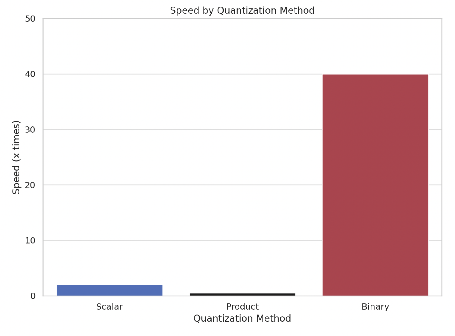
Our results are dramatic: Using BQ will reduce your memory consumption and improve retrieval speeds by up to 40x.
As is the case with other quantization methods, these benefits come at the cost of recall degradation. However, our implementation lets you balance the tradeoff between speed and recall accuracy at time of search, rather than time of index creation.
The rest of this article will cover:
- The importance of binary quantization
- Basic implementation using our Python client
- Benchmark analysis and usage recommendations
What is Binary Quantization?
Binary quantization (BQ) converts any vector embedding of floating point numbers into a vector of binary or boolean values. This feature is an extension of our past work on scalar quantization where we convert float32 to uint8 and then leverage a specific SIMD CPU instruction to perform fast vector comparison.
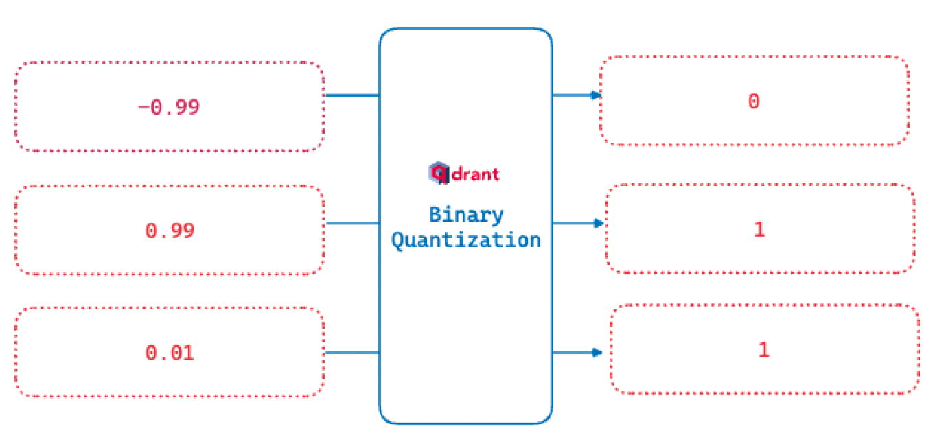
This binarization function is how we convert a range to binary values. All numbers greater than zero are marked as 1. If it’s zero or less, they become 0.
The benefit of reducing the vector embeddings to binary values is that boolean operations are very fast and need significantly less CPU instructions. In exchange for reducing our 32 bit embeddings to 1 bit embeddings we can see up to a 40x retrieval speed up gain!
One of the reasons vector search still works with such a high compression rate is that these large vectors are over-parameterized for retrieval. This is because they are designed for ranking, clustering, and similar use cases, which typically need more information encoded in the vector.
For example, The 1536 dimension OpenAI embedding is worse than Open Source counterparts of 384 dimension at retrieval and ranking. Specifically, it scores 49.25 on the same Embedding Retrieval Benchmark where the Open Source bge-small scores 51.82. This 2.57 points difference adds up quite soon.
Our implementation of quantization achieves a good balance between full, large vectors at ranking time and binary vectors at search and retrieval time. It also has the ability for you to adjust this balance depending on your use case.
Faster search and retrieval
Unlike product quantization, binary quantization does not rely on reducing the search space for each probe. Instead, we build a binary index that helps us achieve large increases in search speed.
HNSW is the approximate nearest neighbor search. This means our accuracy improves up to a point of diminishing returns, as we check the index for more similar candidates. In the context of binary quantization, this is referred to as the oversampling rate.
For example, if oversampling=2.0 and the limit=100, then 200 vectors will first be selected using a quantized index. For those 200 vectors, the full 32 bit vector will be used with their HNSW index to a much more accurate 100 item result set. As opposed to doing a full HNSW search, we oversample a preliminary search and then only do the full search on this much smaller set of vectors.
Improved storage efficiency
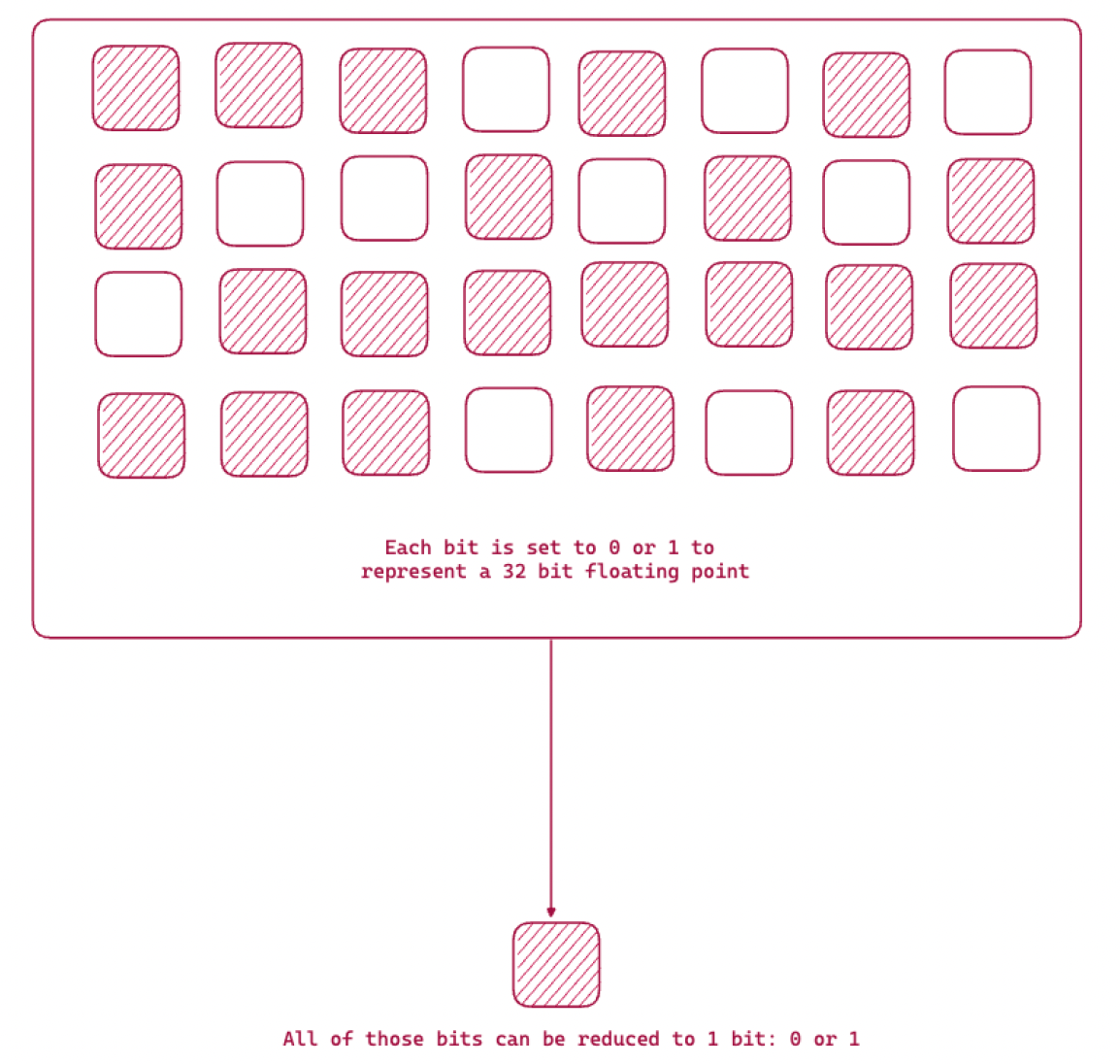
The following diagram shows the binarization function, whereby we reduce 32 bits storage to 1 bit information.
Text embeddings can be over 1024 elements of floating point 32 bit numbers. For example, remember that OpenAI embeddings are 1536 element vectors. This means each vector is 6kB for just storing the vector.
In addition to storing the vector, we also need to maintain an index for faster search and retrieval. Qdrant’s formula to estimate overall memory consumption is:
memory_size = 1.5 * number_of_vectors * vector_dimension * 4 bytes
For 100K OpenAI Embedding (ada-002) vectors we would need 900 Megabytes of RAM and disk space. This consumption can start to add up rapidly as you create multiple collections or add more items to the database.
With binary quantization, those same 100K OpenAI vectors only require 128 MB of RAM. We benchmarked this result using methods similar to those covered in our Scalar Quantization memory estimation.
This reduction in RAM usage is achieved through the compression that happens in the binary conversion. HNSW and quantized vectors will live in RAM for quick access, while original vectors can be offloaded to disk only. For searching, quantized HNSW will provide oversampled candidates, then they will be re-evaluated using their disk-stored original vectors to refine the final results. All of this happens under the hood without any additional intervention on your part.
When should you not use BQ?
Since this method exploits the over-parameterization of embedding, you can expect poorer results for small embeddings i.e. less than 1024 dimensions. With the smaller number of elements, there is not enough information maintained in the binary vector to achieve good results.
You will still get faster boolean operations and reduced RAM usage, but the accuracy degradation might be too high.
Sample implementation
Now that we have introduced you to binary quantization, let’s try our a basic implementation. In this example, we will be using OpenAI and Cohere with Qdrant.
Create a collection with Binary Quantization enabled
Here is what you should do at indexing time when you create the collection:
- We store all the “full” vectors on disk.
- Then we set the binary embeddings to be in RAM.
By default, both the full vectors and BQ get stored in RAM. We move the full vectors to disk because this saves us memory and allows us to store more vectors in RAM. By doing this, we explicitly move the binary vectors to memory by setting always_ram=True.
from qdrant_client import QdrantClient

#collect to our Qdrant Server
client = QdrantClient(
    url="http://localhost:6333",
    prefer_grpc=True,
)

#Create the collection to hold our embeddings
# on_disk=True and the quantization_config are the areas to focus on
collection_name = "binary-quantization"
if not client.collection_exists(collection_name):
    client.create_collection(
        collection_name=f"{collection_name}",
        vectors_config=models.VectorParams(
            size=1536,
            distance=models.Distance.DOT,
            on_disk=True,
        ),
        optimizers_config=models.OptimizersConfigDiff(
            default_segment_number=5,
        ),
        hnsw_config=models.HnswConfigDiff(
        m=0,
        ),
        quantization_config=models.BinaryQuantization(
            binary=models.BinaryQuantizationConfig(always_ram=True),
        ),
    )
What is happening in the HnswConfig?
We’re setting m to 0 i.e. disabling the HNSW graph construction. This allows faster uploads of vectors and payloads. We will turn it back on down below, once all the data is loaded.
Next, we upload our vectors to this and then enable the graph construction:
batch_size = 10000
client.upload_collection(
    collection_name=collection_name,
    ids=range(len(dataset)),
    vectors=dataset["openai"],
    payload=[
        {"text": x} for x in dataset["text"]
    ],
    parallel=10, # based on the machine
)
Enable HNSW graph construction again:
client.update_collection(
    collection_name=f"{collection_name}",
    hnsw_config=models.HnswConfigDiff(
        m=16,
    ,
)
Configure the search parameters:
When setting search parameters, we specify that we want to use oversampling and rescore. Here is an example snippet:
client.search(
    collection_name="{collection_name}",
    query_vector=[0.2, 0.1, 0.9, 0.7, ...],
    search_params=models.SearchParams(
        quantization=models.QuantizationSearchParams(
            ignore=False,
            rescore=True,
            oversampling=2.0,
        )
    )
)
After Qdrant pulls the oversampled vectors set, the full vectors which will be, say 1536 dimensions for OpenAI will then be pulled up from disk. Qdrant computes the nearest neighbor with the query vector and returns the accurate, rescored order. This method produces much more accurate results. We enabled this by setting rescore=True.
These two parameters are how you are going to balance speed versus accuracy. The larger the size of your oversample, the more items you need to read from disk and the more elements you have to search with the relatively slower full vector index. On the other hand, doing this will produce more accurate results.
If you have lower accuracy requirements you can even try doing a small oversample without rescoring. Or maybe, for your data set combined with your accuracy versus speed requirements you can just search the binary index and no rescoring, i.e. leaving those two parameters out of the search query.
Benchmark results
We retrieved some early results on the relationship between limit and oversampling using the the DBPedia OpenAI 1M vector dataset. We ran all these experiments on a Qdrant instance where 100K vectors were indexed and used 100 random queries.
We varied the 3 parameters that will affect query time and accuracy: limit, rescore and oversampling. We offer these as an initial exploration of this new feature. You are highly encouraged to reproduce these experiments with your datasets.
Aside: Since this is a new innovation in vector databases, we are keen to hear feedback and results. Join our Discord server for further discussion!
Oversampling: In the figure below, we illustrate the relationship between recall and number of candidates:
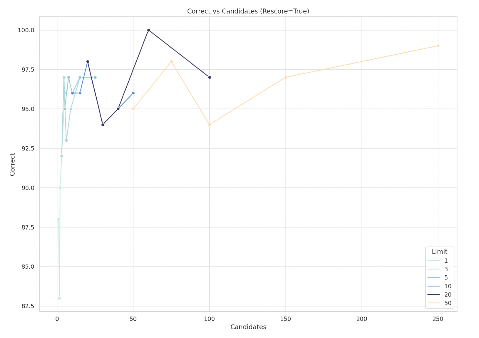
We see that “correct” results i.e. recall increases as the number of potential “candidates” increase (limit x oversampling). To highlight the impact of changing the limit, different limit values are broken apart into different curves. For example, we see that the lowest recall for limit 50 is around 94 correct, with 100 candidates. This also implies we used an oversampling of 2.0
As oversampling increases, we see a general improvement in results – but that does not hold in every case.
Rescore: As expected, rescoring increases the time it takes to return a query. We also repeated the experiment with oversampling except this time we looked at how rescore impacted result accuracy.
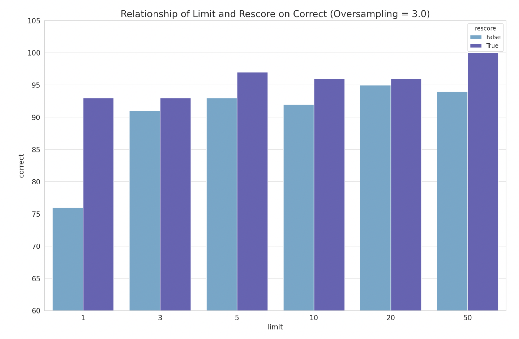
Limit: We experiment with limits from Top 1 to Top 50 and we are able to get to 100% recall at limit 50, with rescore=True, in an index with 100K vectors.
Recommendations
Quantization gives you the option to make tradeoffs against other parameters: Dimension count/embedding size Throughput and Latency requirements Recall requirements
If you’re working with OpenAI or Cohere embeddings, we recommend the following oversampling settings:
| Method | Dimensionality | Test Dataset | Recall | Oversampling |
|---|---|---|---|---|
| OpenAI text-embedding-3-large | 3072 | DBpedia 1M | 0.9966 | 3x |
| OpenAI text-embedding-3-small | 1536 | DBpedia 100K | 0.9847 | 3x |
| OpenAI text-embedding-3-large | 1536 | DBpedia 1M | 0.9826 | 3x |
| OpenAI text-embedding-ada-002 | 1536 | DbPedia 1M | 0.98 | 4x |
| Gemini | 768 | No Open Data | 0.9563 | 3x |
| Mistral Embed | 768 | No Open Data | 0.9445 | 3x |
If you determine that binary quantization is appropriate for your datasets and queries then we suggest the following:
- Binary Quantization with always_ram=True
- Vectors stored on disk
- Oversampling=2.0 (or more)
- Rescore=True
What’s next?
Binary quantization is exceptional if you need to work with large volumes of data under high recall expectations. You can try this feature either by spinning up a Qdrant container image locally or, having us create one for you through a free account in our cloud hosted service.
The article gives examples of datasets and configuration you can use to get going. Our documentation covers adding large datasets to Qdrant to your Qdrant instance as well as more quantization methods.
If you have any feedback, drop us a note on Twitter or LinkedIn to tell us about your results. Join our lively Discord Server if you want to discuss BQ with like-minded people!