
Data Structures 101
Those who took programming courses might remember that there is no such thing as a universal data structure. Some structures are good at accessing elements by index (like arrays), while others shine in terms of insertion efficiency (like linked lists).
Hardware-optimized data structure
However, when we move from theoretical data structures to real-world systems, and particularly in performance-critical areas such as vector search, things become more complex. Big-O notation provides a good abstraction, but it doesn’t account for the realities of modern hardware: cache misses, memory layout, disk I/O, and other low-level considerations that influence actual performance.
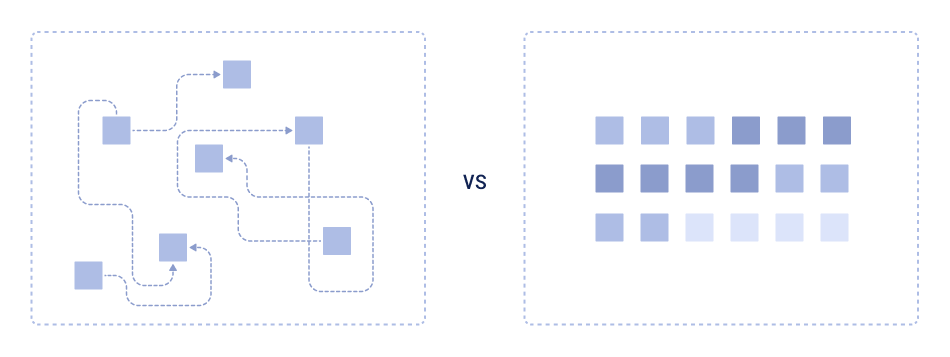
From the perspective of hardware efficiency, the ideal data structure is a contiguous array of bytes that can be read sequentially in a single thread. This scenario allows hardware optimizations like prefetching, caching, and branch prediction to operate at their best.
However, real-world use cases require more complex structures to perform various operations like insertion, deletion, and search. These requirements increase complexity and introduce performance trade-offs.
Mutability
One of the most significant challenges when working with data structures is ensuring mutability — the ability to change the data structure after it’s created, particularly with fast update operations.
Let’s consider a simple example: we want to iterate over items in sorted order. Without a mutability requirement, we can use a simple array and sort it once. This is very close to our ideal scenario. We can even put the structure on disk - which is trivial for an array.
However, if we need to insert an item into this array, things get more complicated. Inserting into a sorted array requires shifting all elements after the insertion point, which leads to linear time complexity for each insertion, which is not acceptable for many applications.
To handle such cases, more complex structures like B-trees come into play. B-trees are specifically designed to optimize both insertion and read operations for large data sets. However, they sacrifice the raw speed of array reads for better insertion performance.
Here’s a benchmark that illustrates the difference between iterating over a plain array and a BTreeSet in Rust:
use std::collections::BTreeSet;
use rand::Rng;

fn main() {
    // Benchmark plain vector VS btree in a task of iteration over all elements
    let mut rand = rand::thread_rng();
    let vector: Vec<_> = (0..1000000).map(|_| rand.gen::<u64>()).collect();
    let btree: BTreeSet<_> = vector.iter().copied().collect();

    {
        let mut sum = 0;
        for el in vector {
            sum += el;
        }
    } // Elapsed: 850.924µs

    {
        let mut sum = 0;
        for el in btree {
            sum += el;
        }
    } // Elapsed: 5.213025ms, ~6x slower

}
Vector databases, like Qdrant, have to deal with a large variety of data structures. If we could make them immutable, it would significantly improve performance and optimize memory usage.
How Does Immutability Help?
A large part of the immutable advantage comes from the fact that we know the exact data we need to put into the structure even before we start building it. The simplest example is a sorted array: we would know exactly how many elements we have to put into the array so we can allocate the exact amount of memory once.
More complex data structures might require additional statistics to be collected before the structure is built. A Qdrant-related example of this is Scalar Quantization: in order to select proper quantization levels, we have to know the distribution of the data.
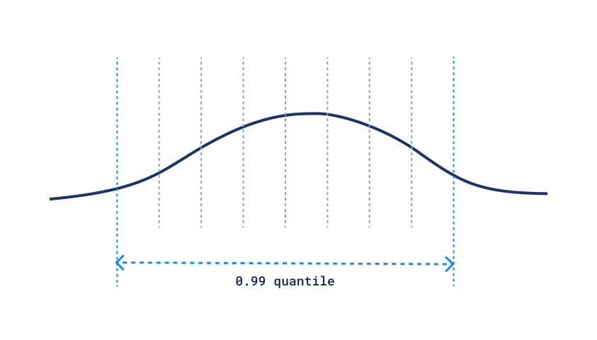
Scalar Quantization Quantile
Computing this distribution requires knowing all the data in advance, but once we have it, applying scalar quantization is a simple operation.
Let’s take a look at a non-exhaustive list of data structures and potential improvements we can get from making them immutable:
| Function | Mutable Data Structure | Immutable Alternative | Potential improvements |
|---|---|---|---|
| Read by index | Array | Fixed chunk of memory | Allocate exact amount of memory |
| Vector Storage | Array or Arrays | Memory-mapped file | Offload data to disk |
| Read sorted ranges | B-Tree | Sorted Array | Store all data close, avoid cache misses |
| Read by key | Hash Map | Hash Map with Perfect Hashing | Avoid hash collisions |
| Get documents by keyword | Inverted Index | Inverted Index with Sortedand BitPacked Postings | Less memory usage, faster search |
| Vector Search | HNSW graph | HNSW graph withpayload-aware connections | Better precision with filters |
| Tenant Isolation | Vector Storage | Defragmented Vector Storage | Faster access to on-disk data |
For more info on payload-aware connections in HNSW, read our previous article.
This time around, we will focus on the latest additions to Qdrant:
- the immutable hash map with perfect hashing
- defragmented vector storage.
Perfect Hashing
A hash table is one of the most commonly used data structures implemented in almost every programming language, including Rust. It provides fast access to elements by key, with an average time complexity of O(1) for read and write operations.
There is, however, the assumption that should be satisfied for the hash table to work efficiently: hash collisions should not cause too much overhead. In a hash table, each key is mapped to a “bucket,” a slot where the value is stored. When different keys map to the same bucket, a collision occurs.
In regular mutable hash tables, minimization of collisions is achieved by:
- making the number of buckets bigger so the probability of collision is lower
- using a linked list or a tree to store multiple elements with the same hash
However, these strategies have overheads, which become more significant if we consider using high-latency storage like disk.
Indeed, every read operation from disk is several orders of magnitude slower than reading from RAM, so we want to know the correct location of the data from the first attempt.
In order to achieve this, we can use a so-called minimal perfect hash function (MPHF). This special type of hash function is constructed specifically for a given set of keys, and it guarantees no collisions while using minimal amount of buckets.
In Qdrant, we decided to use fingerprint-based minimal perfect hash function implemented in the ph crate 🦀 by Piotr Beling. According to our benchmarks, using the perfect hash function does introduce some overhead in terms of hashing time, but it significantly reduces the time for the whole operation:
| Volume | ph::Function | std::hash::Hash | HashMap::get |
|---|---|---|---|
| 1000 | 60ns | ~20ns | 34ns |
| 100k | 90ns | ~20ns | 220ns |
| 10M | 238ns | ~20ns | 500ns |
Even thought the absolute time for hashing is higher, the time for the whole operation is lower, because PHF guarantees no collisions. The difference is even more significant when we consider disk read time, which might up to several milliseconds (10^6 ns).
PHF RAM size scales linearly for ph::Function: 3.46 kB for 10k elements, 119MB for 350M elements.
The construction time required to build the hash function is surprisingly low, and we only need to do it once:
| Volume | ph::Function (construct) | PHF size | Size of int64 keys (for reference) |
|---|---|---|---|
| 1M | 52ms | 0.34Mb | 7.62Mb |
| 100M | 7.4s | 33.7Mb | 762.9Mb |
The usage of PHF in Qdrant lets us minimize the latency of cold reads, which is especially important for large-scale multi-tenant systems. With PHF, it is enough to read a single page from a disk to get the exact location of the data.
Defragmentation
When you read data from a disk, you almost never read a single byte. Instead, you read a page, which is a fixed-size chunk of data. On many systems, the page size is 4KB, which means that every read operation will read 4KB of data, even if you only need a single byte.
Vector search, on the other hand, requires reading a lot of small vectors, which might create a large overhead. It is especially noticeable if we use binary quantization, where the size of even large OpenAI 1536d vectors is compressed down to 192 bytes.
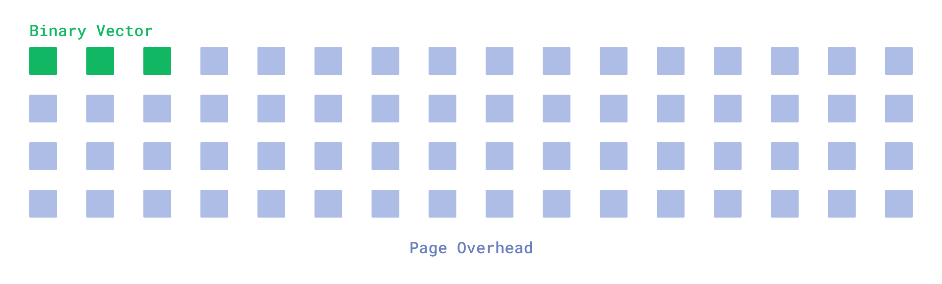
Overhead when reading single vector
That means if the vectors we access during the search are randomly scattered across the disk, we will have to read 4KB for each vector, which is 20 times more than the actual data size.
There is, however, a simple way to avoid this overhead: defragmentation. If we knew some additional information about the data, we could combine all relevant vectors into a single page.
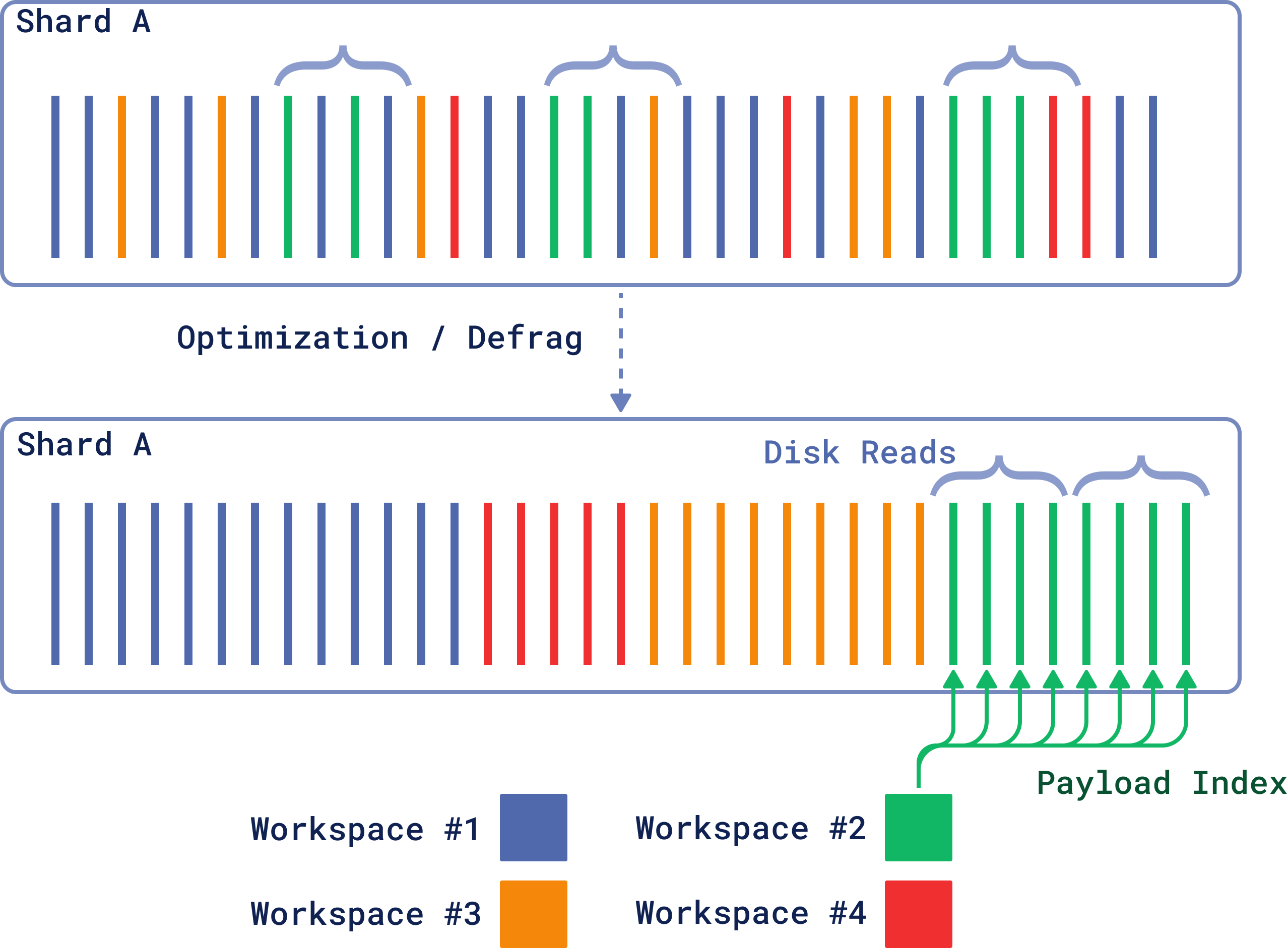
Defragmentation
This additional information is available to Qdrant via the payload index.
By specifying the payload index, which is going to be used for filtering most of the time, we can put all vectors with the same payload together. This way, reading a single page will also read nearby vectors, which will be used in the search.
This approach is especially efficient for multi-tenant systems, where only a small subset of vectors is actively used for search. The capacity of such a deployment is typically defined by the size of the hot subset, which is much smaller than the total number of vectors.
Grouping relevant vectors together allows us to optimize the size of the hot subset by avoiding caching of irrelevant data. The following benchmark data compares RPS for defragmented and non-defragmented storage:
| % of hot subset | Tenant Size (vectors) | RPS, Non-defragmented | RPS, Defragmented |
|---|---|---|---|
| 2.5% | 50k | 1.5 | 304 |
| 12.5% | 50k | 0.47 | 279 |
| 25% | 50k | 0.4 | 63 |
| 50% | 50k | 0.3 | 8 |
| 2.5% | 5k | 56 | 490 |
| 12.5% | 5k | 5.8 | 488 |
| 25% | 5k | 3.3 | 490 |
| 50% | 5k | 3.1 | 480 |
| 75% | 5k | 2.9 | 130 |
| 100% | 5k | 2.7 | 95 |
Dataset size: 2M 768d vectors (~6Gb Raw data), binary quantization, 650Mb of RAM limit. All benchmarks are made with minimal RAM allocation to demonstrate disk cache efficiency.
As you can see, the biggest impact is on the small tenant size, where defragmentation allows us to achieve 100x more RPS. Of course, the real-world impact of defragmentation depends on the specific workload and the size of the hot subset, but enabling this feature can significantly improve the performance of Qdrant.
Please find more details on how to enable defragmentation in the indexing documentation.
Updating Immutable Data Structures
One may wonder how Qdrant allows updating collection data if everything is immutable. Indeed, Qdrant API allows the change of any vector or payload at any time, so from the user’s perspective, the whole collection is mutable at any time.
As it usually happens with every decent magic trick, the secret is disappointingly simple: not all data in Qdrant is immutable. In Qdrant, storage is divided into segments, which might be either mutable or immutable. New data is always written to the mutable segment, which is later converted to the immutable one by the optimization process.
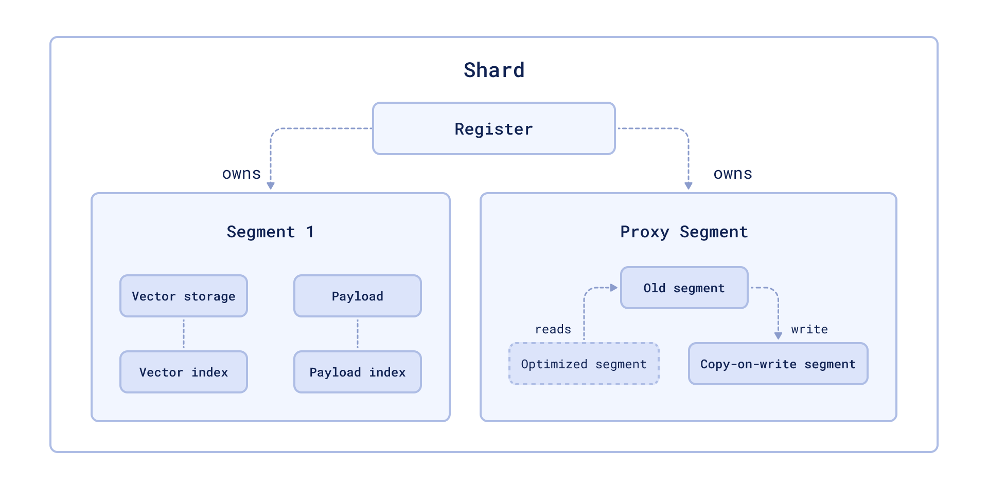
Optimization process
If we need to update the data in the immutable or currenly optimized segment, instead of changing the data in place, we perform a copy-on-write operation, move the data to the mutable segment, and update it there.
Data in the original segment is marked as deleted, and later vacuumed by the optimization process.
Downsides and How to Compensate
While immutable data structures are great for read-heavy operations, they come with trade-offs:
- Higher update costs: Immutable structures are less efficient for updates. The amortized time complexity might be the same as mutable structures, but the constant factor is higher.
- Rebuilding overhead: In some cases, we may need to rebuild indices or structures for the same data more than once.
- Read-heavy workloads: Immutability assumes a search-heavy workload, which is typical for search engines but not for all applications.
In Qdrant, we mitigate these downsides by allowing the user to adapt the system to their specific workload. For example, changing the default size of the segment might help to reduce the overhead of rebuilding indices.
In extreme cases, multi-segment storage can act as a single segment, falling back to the mutable data structure when needed.
Conclusion
Immutable data structures, while tricky to implement correctly, offer significant performance gains, especially for read-heavy systems like search engines. They allow us to take full advantage of hardware optimizations, reduce memory overhead, and improve cache performance.
In Qdrant, the combination of techniques like perfect hashing and defragmentation brings further benefits, making our vector search operations faster and more efficient. While there are trade-offs, the flexibility of Qdrant’s architecture — including segment-based storage — allows us to balance the best of both worlds.