Any* Embedding Model Can Become a Late Interaction Model... If You Give It a Chance!
Kacper Łukawski
·August 14, 2024

* At least any open-source model, since you need access to its internals.
You Can Adapt Dense Embedding Models for Late Interaction
Qdrant 1.10 introduced support for multi-vector representations, with late interaction being a prominent example of this model. In essence, both documents and queries are represented by multiple vectors, and identifying the most relevant documents involves calculating a score based on the similarity between the corresponding query and document embeddings. If you’re not familiar with this paradigm, our updated Hybrid Search article explains how multi-vector representations can enhance retrieval quality.
Figure 1: We can visualize late interaction between corresponding document-query embedding pairs.
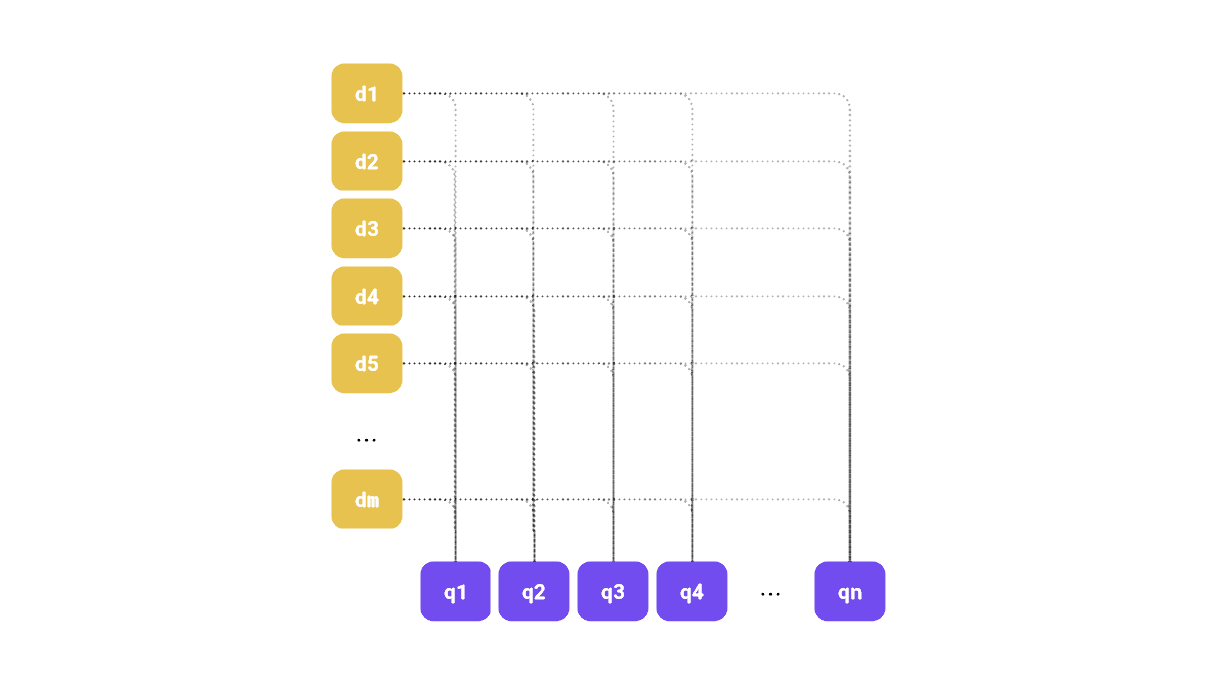
There are many specialized late interaction models, such as ColBERT, but it appears that regular dense embedding models can also be effectively utilized in this manner.
In this study, we will demonstrate that standard dense embedding models, traditionally used for single-vector representations, can be effectively adapted for late interaction scenarios using output token embeddings as multi-vector representations.
By testing out retrieval with Qdrant’s multi-vector feature, we will show that these models can rival or surpass specialized late interaction models in retrieval performance, while offering lower complexity and greater efficiency. This work redefines the potential of dense models in advanced search pipelines, presenting a new method for optimizing retrieval systems.
Understanding Embedding Models
The inner workings of embedding models might be surprising to some. The model doesn’t operate directly on the input text; instead, it requires a tokenization step to convert the text into a sequence of token identifiers. Each token identifier is then passed through an embedding layer, which transforms it into a dense vector. Essentially, the embedding layer acts as a lookup table that maps token identifiers to dense vectors. These vectors are then fed into the transformer model as input.
Figure 2: The tokenization step, which takes place before vectors are added to the transformer model.
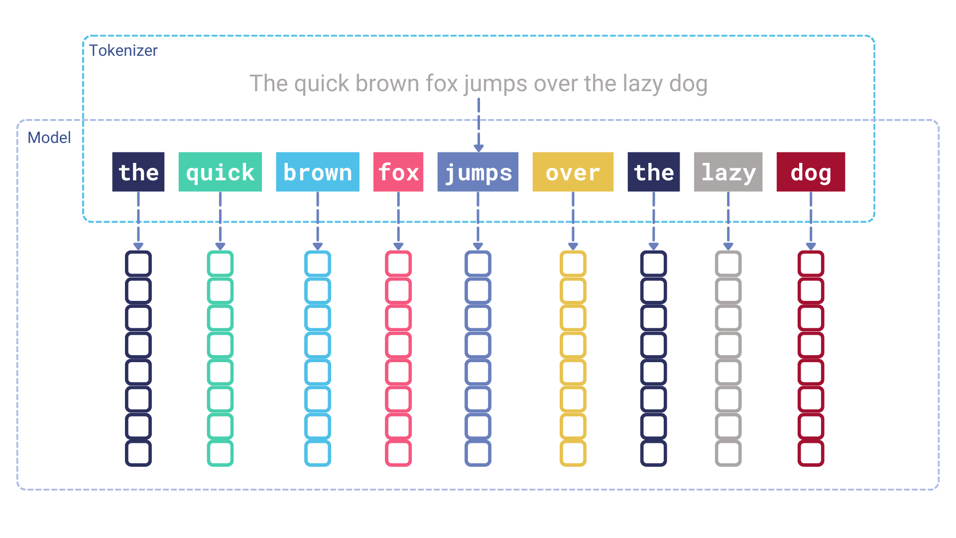
The input token embeddings are context-free and are learned during the model’s training process. This means that each token always receives the same embedding, regardless of its position in the text. At this stage, the token embeddings are unaware of the context in which they appear. It is the transformer model’s role to contextualize these embeddings.
Much has been discussed about the role of attention in transformer models, but in essence, this mechanism is responsible for capturing cross-token relationships. Each transformer module takes a sequence of token embeddings as input and produces a sequence of output token embeddings. Both sequences are of the same length, with each token embedding being enriched by information from the other token embeddings at the current step.
Figure 3: The mechanism that produces a sequence of output token embeddings.
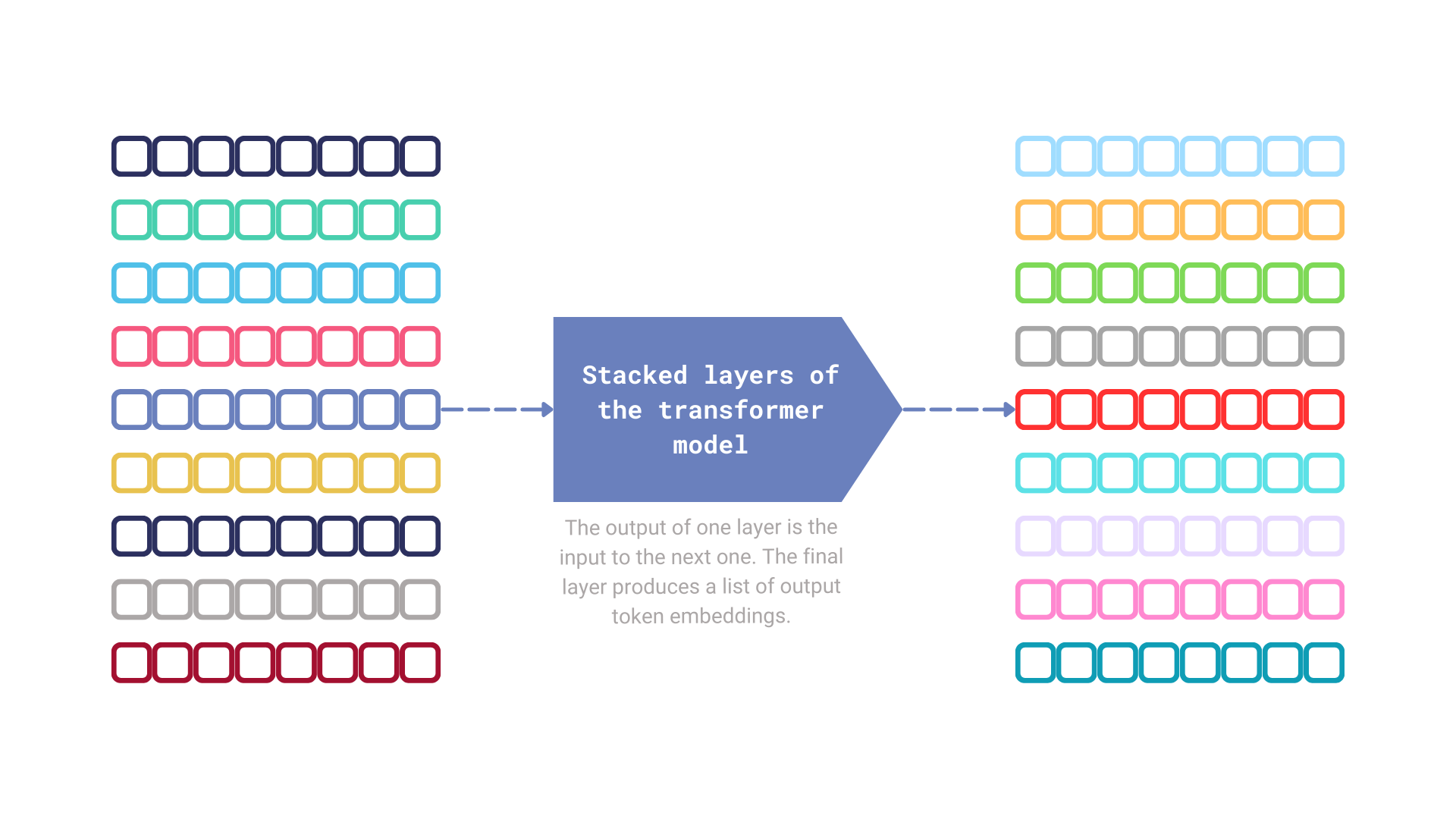
Figure 4: The final step performed by the embedding model is pooling the output token embeddings to generate a single vector representation of the input text.
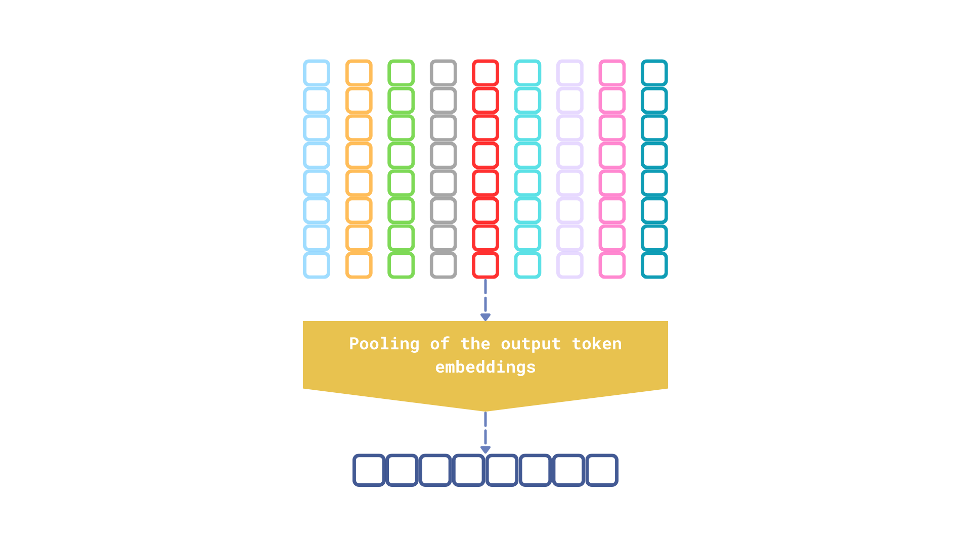
There are several pooling strategies, but regardless of which one a model uses, the output is always a single vector representation, which inevitably loses some information about the input. It’s akin to giving someone detailed, step-by-step directions to the nearest grocery store versus simply pointing in the general direction. While the vague direction might suffice in some cases, the detailed instructions are more likely to lead to the desired outcome.
Using Output Token Embeddings for Multi-Vector Representations
We often overlook the output token embeddings, but the fact is—they also serve as multi-vector representations of the input text. So, why not explore their use in a multi-vector retrieval model, similar to late interaction models?
Experimental Findings
We conducted several experiments to determine whether output token embeddings could be effectively used in place of traditional late interaction models. The results are quite promising.
| Dataset | Model | Experiment | NDCG@10 |
|---|---|---|---|
| SciFact | prithivida/Splade_PP_en_v1 | sparse vectors | 0.70928 |
colbert-ir/colbertv2.0 | late interaction model | 0.69579 | |
all-MiniLM-L6-v2 | single dense vector representation | 0.64508 | |
| output token embeddings | 0.70724 | ||
BAAI/bge-small-en | single dense vector representation | 0.68213 | |
| output token embeddings | 0.73696 | ||
| NFCorpus | prithivida/Splade_PP_en_v1 | sparse vectors | 0.34166 |
colbert-ir/colbertv2.0 | late interaction model | 0.35036 | |
all-MiniLM-L6-v2 | single dense vector representation | 0.31594 | |
| output token embeddings | 0.35779 | ||
BAAI/bge-small-en | single dense vector representation | 0.29696 | |
| output token embeddings | 0.37502 | ||
| ArguAna | prithivida/Splade_PP_en_v1 | sparse vectors | 0.47271 |
colbert-ir/colbertv2.0 | late interaction model | 0.44534 | |
all-MiniLM-L6-v2 | single dense vector representation | 0.50167 | |
| output token embeddings | 0.45997 | ||
BAAI/bge-small-en | single dense vector representation | 0.58857 | |
| output token embeddings | 0.57648 | ||
The source code for these experiments is open-source and utilizes beir-qdrant, an integration of Qdrant with the BeIR library. While this package is not officially maintained by the Qdrant team, it may prove useful for those interested in experimenting with various Qdrant configurations to see how they impact retrieval quality. All experiments were conducted using Qdrant in exact search mode, ensuring the results are not influenced by approximate search.
Even the simple all-MiniLM-L6-v2 model can be applied in a late interaction model fashion, resulting in a positive impact on retrieval quality. However, the best results were achieved with the BAAI/bge-small-en model, which outperformed both sparse and late interaction models.
It’s important to note that ColBERT has not been trained on BeIR datasets, making its performance fully out of domain. Nevertheless, the all-MiniLM-L6-v2 training dataset also lacks any BeIR data, yet it still performs remarkably well.
Comparative Analysis of Dense vs. Late Interaction Models
The retrieval quality speaks for itself, but there are other important factors to consider.
The traditional dense embedding models we tested are less complex than late interaction or sparse models. With fewer parameters, these models are expected to be faster during inference and more cost-effective to maintain. Below is a comparison of the models used in the experiments:
| Model | Number of parameters |
|---|---|
prithivida/Splade_PP_en_v1 | 109,514,298 |
colbert-ir/colbertv2.0 | 109,580,544 |
BAAI/bge-small-en | 33,360,000 |
all-MiniLM-L6-v2 | 22,713,216 |
One argument against using output token embeddings is the increased storage requirements compared to ColBERT-like models. For instance, the all-MiniLM-L6-v2 model produces 384-dimensional output token embeddings, which is three times more than the 128-dimensional embeddings generated by ColBERT-like models. This increase not only leads to higher memory usage but also impacts the computational cost of retrieval, as calculating distances takes more time. Mitigating this issue through vector compression would make a lot of sense.
Exploring Quantization for Multi-Vector Representations
Binary quantization is generally more effective for high-dimensional vectors, making the all-MiniLM-L6-v2 model, with its relatively low-dimensional outputs, less ideal for this approach. However, scalar quantization appeared to be a viable alternative. The table below summarizes the impact of quantization on retrieval quality.
| Dataset | Model | Experiment | NDCG@10 |
|---|---|---|---|
| SciFact | all-MiniLM-L6-v2 | output token embeddings | 0.70724 |
| output token embeddings (uint8) | 0.70297 | ||
| NFCorpus | all-MiniLM-L6-v2 | output token embeddings | 0.35779 |
| output token embeddings (uint8) | 0.35572 | ||
It’s important to note that quantization doesn’t always preserve retrieval quality at the same level, but in this case, scalar quantization appears to have minimal impact on retrieval performance. The effect is negligible, while the memory savings are substantial.
We managed to maintain the original quality while using four times less memory. Additionally, a quantized vector requires 384 bytes, compared to ColBERT’s 512 bytes. This results in a 25% reduction in memory usage, with retrieval quality remaining nearly unchanged.
Practical Application: Enhancing Retrieval with Dense Models
If you’re using one of the sentence transformer models, the output token embeddings are calculated by default. While a single vector representation is more efficient in terms of storage and computation, there’s no need to discard the output token embeddings. According to our experiments, these embeddings can significantly enhance retrieval quality. You can store both the single vector and the output token embeddings in Qdrant, using the single vector for the initial retrieval step and then reranking the results with the output token embeddings.
Figure 5: A single model pipeline that relies solely on the output token embeddings for reranking.
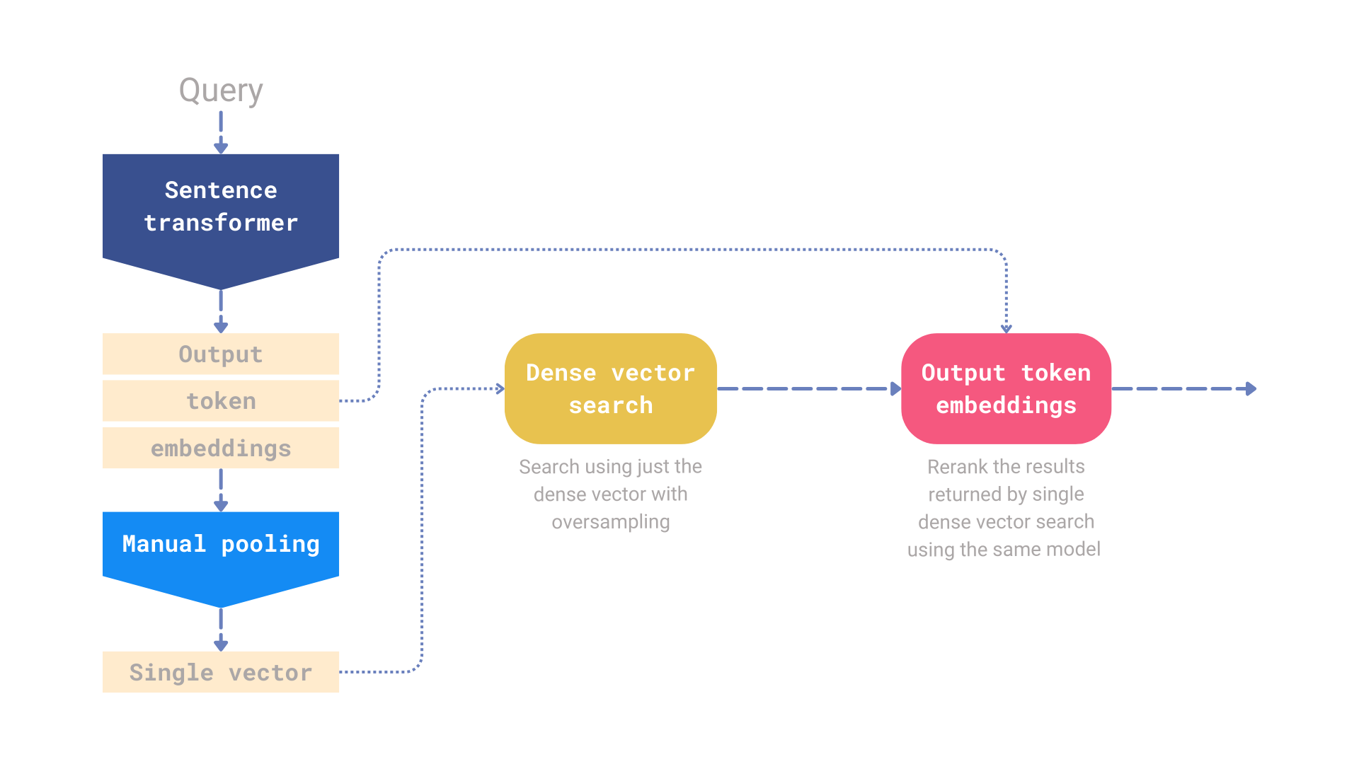
To demonstrate this concept, we implemented a simple reranking pipeline in Qdrant. This pipeline uses a dense embedding model for the initial oversampled retrieval and then relies solely on the output token embeddings for the reranking step.
Single Model Retrieval and Reranking Benchmarks
Our tests focused on using the same model for both retrieval and reranking. The reported metric is NDCG@10. In all tests, we applied an oversampling factor of 5x, meaning the retrieval step returned 50 results, which were then narrowed down to 10 during the reranking step. Below are the results for some of the BeIR datasets:
| Dataset | all-miniLM-L6-v2 | BAAI/bge-small-en | ||
|---|---|---|---|---|
| dense embeddings only | dense + reranking | dense embeddings only | dense + reranking | |
| SciFact | 0.64508 | 0.70293 | 0.68213 | 0.73053 |
| NFCorpus | 0.31594 | 0.34297 | 0.29696 | 0.35996 |
| ArguAna | 0.50167 | 0.45378 | 0.58857 | 0.57302 |
| Touche-2020 | 0.16904 | 0.19693 | 0.13055 | 0.19821 |
| TREC-COVID | 0.47246 | 0.6379 | 0.45788 | 0.53539 |
| FiQA-2018 | 0.36867 | 0.41587 | 0.31091 | 0.39067 |
The source code for the benchmark is publicly available, and you can find it in the repository of the beir-qdrant package.
Overall, adding a reranking step using the same model typically improves retrieval quality. However, the quality of various late interaction models is often reported based on their reranking performance when BM25 is used for the initial retrieval. This experiment aimed to demonstrate how a single model can be effectively used for both retrieval and reranking, and the results are quite promising.
Now, let’s explore how to implement this using the new Query API introduced in Qdrant 1.10.
Setting Up Qdrant for Late Interaction
The new Query API in Qdrant 1.10 enables the construction of even more complex retrieval pipelines. We can use the single vector created after pooling for the initial retrieval step and then rerank the results using the output token embeddings.
Assuming the collection is named my-collection and is configured to store two named vectors: dense-vector and output-token-embeddings, here’s how such a collection could be created in Qdrant:
from qdrant_client import QdrantClient, models

client = QdrantClient("http://localhost:6333")

client.create_collection(
    collection_name="my-collection",
    vectors_config={
        "dense-vector": models.VectorParams(
            size=384,
            distance=models.Distance.COSINE,
        ),
        "output-token-embeddings": models.VectorParams(
            size=384,
            distance=models.Distance.COSINE,
            multivector_config=models.MultiVectorConfig(
                comparator=models.MultiVectorComparator.MAX_SIM
            ),
        ),
    }
)
Both vectors are of the same size since they are produced by the same all-MiniLM-L6-v2 model.
from sentence_transformers import SentenceTransformer

model = SentenceTransformer("all-MiniLM-L6-v2")
Now, instead of using the search API with just a single dense vector, we can create a reranking pipeline. First, we retrieve 50 results using the dense vector, and then we rerank them using the output token embeddings to obtain the top 10 results.
query = "What else can be done with just all-MiniLM-L6-v2 model?"

client.query_points(
    collection_name="my-collection",
    prefetch=[
        # Prefetch the dense embeddings of the top-50 documents
        models.Prefetch(
            query=model.encode(query).tolist(),
            using="dense-vector",
            limit=50,
        )
    ],
    # Rerank the top-50 documents retrieved by the dense embedding model
    # and return just the top-10. Please note we call the same model, but
    # we ask for the token embeddings by setting the output_value parameter.
    query=model.encode(query, output_value="token_embeddings").tolist(),
    using="output-token-embeddings",
    limit=10,
)
Try the Experiment Yourself
In a real-world scenario, you might take it a step further by first calculating the token embeddings and then performing pooling to obtain the single vector representation. This approach allows you to complete everything in a single pass.
The simplest way to start experimenting with building complex reranking pipelines in Qdrant is by using the forever-free cluster on Qdrant Cloud and reading Qdrant’s documentation.
The source code for these experiments is open-source and uses beir-qdrant, an integration of Qdrant with the BeIR library.
Future Directions and Research Opportunities
The initial experiments using output token embeddings in the retrieval process have yielded promising results. However, we plan to conduct further benchmarks to validate these findings and explore the incorporation of sparse methods for the initial retrieval. Additionally, we aim to investigate the impact of quantization on multi-vector representations and its effects on retrieval quality. Finally, we will assess retrieval speed, a crucial factor for many applications.


