Fine-Tuning Sparse Embeddings for E-Commerce Search | Part 1: Why Sparse Embeddings Beat BM25
Thierry Damiba
·March 09, 2026

This is Part 1 of a 5-part series on fine-tuning sparse embeddings for e-commerce search. We’ll go from “why bother?” to a production system that beats BM25 by 29%.
Series:
- Part 1: Why Sparse Embeddings Beat BM25 (here)
- Part 2: Training on Modal
- Part 3: Evaluation & Hard Negatives
- Part 4: Specialization vs Generalization
- Part 5: From Research to Product
Search “iPhone 15 Pro Max 256GB” on a dense embedding system and it happily returns the 128GB model. The semantic similarity is high - it’s the same phone! But the customer specified 256GB for a reason. In e-commerce, the details aren’t noise. They’re the whole point.
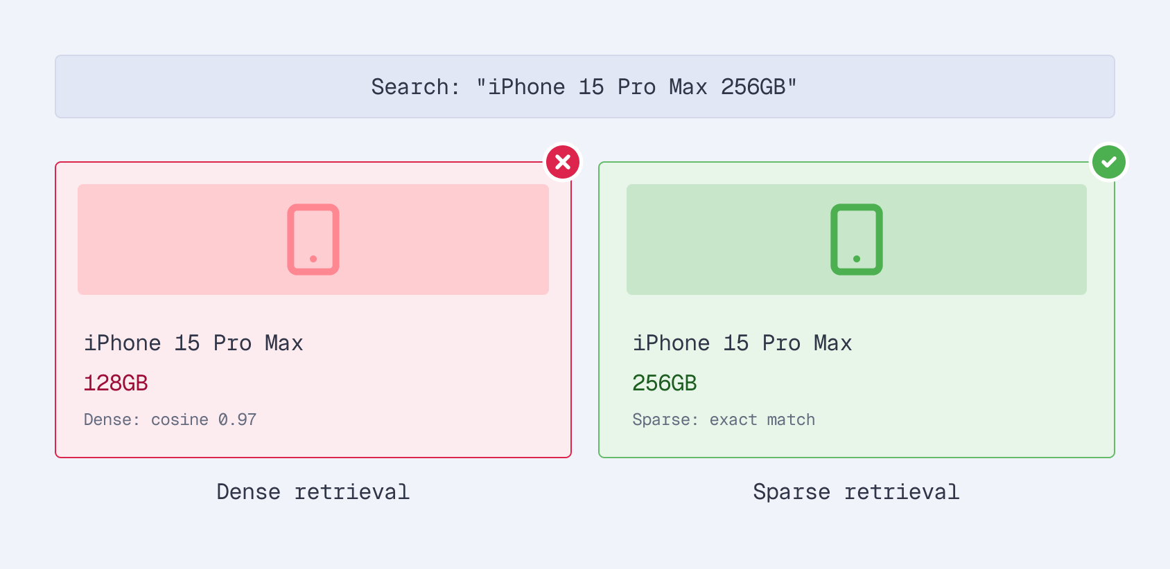
This is the gap that sparse embeddings fill. And with fine-tuning, they fill it dramatically well - we achieved a 29% improvement over BM25 on Amazon’s ESCI dataset, one of the largest public e-commerce search benchmarks.
In this series, we’ll build the entire system: data loading, GPU training on Modal, evaluation with Qdrant, and hard negative mining. The full code is on GitHub and the fine-tuned models are on HuggingFace. If you want to skip the walkthrough and fine-tune on your own data, the sparse-finetune CLI runs the entire pipeline with one command. But first, let’s understand why sparse embeddings are the right tool for e-commerce search.
The Problem with Dense Embeddings in E-Commerce
Dense embeddings (the kind you get from OpenAI, Cohere, or a fine-tuned sentence transformer) compress text into a fixed-size vector, typically 384 to 1536 dimensions, all non-zero. They’re excellent at capturing semantic meaning. “Running shoes” and “jogging sneakers” land close together in the embedding space.
But this strength becomes a weakness in e-commerce:
Exact matches get blurred. When every dimension carries a non-zero value, the model prioritizes broad semantic similarity over exact term matching. SKU numbers, model names, specific sizes - these critical differentiators get averaged into the same neighborhood as similar-but-wrong products.
Retrieval is approximate. At scale, dense vectors require Approximate Nearest Neighbor (ANN) indexes like HNSW. The “approximate” part means you’re trading recall for speed. For search, where missing a relevant product means a lost sale, this tradeoff hurts.
Results are opaque. Why did product X rank above product Y? With dense embeddings, you can’t say. The 768-dimensional vector offers no interpretability. When a merchandising team asks why a product isn’t showing up, you’re stuck.
Enter Sparse Embeddings
Sparse embeddings take a fundamentally different approach. Instead of compressing text into a small, dense vector, they project it onto a large vocabulary space - typically 30,000+ dimensions (one per token in the vocabulary). But only 100-300 of those dimensions are non-zero.
| Dense | Sparse | |
|---|---|---|
| Vector size | 384-1536 dims | ~30,000 dims |
| Non-zero values | All dimensions carry a value | 100-300 terms |
| Index type | ANN (HNSW) | Inverted index |
| Exact matching | Weak | Strong |
| Interpretability | Black box | Per-term weights |
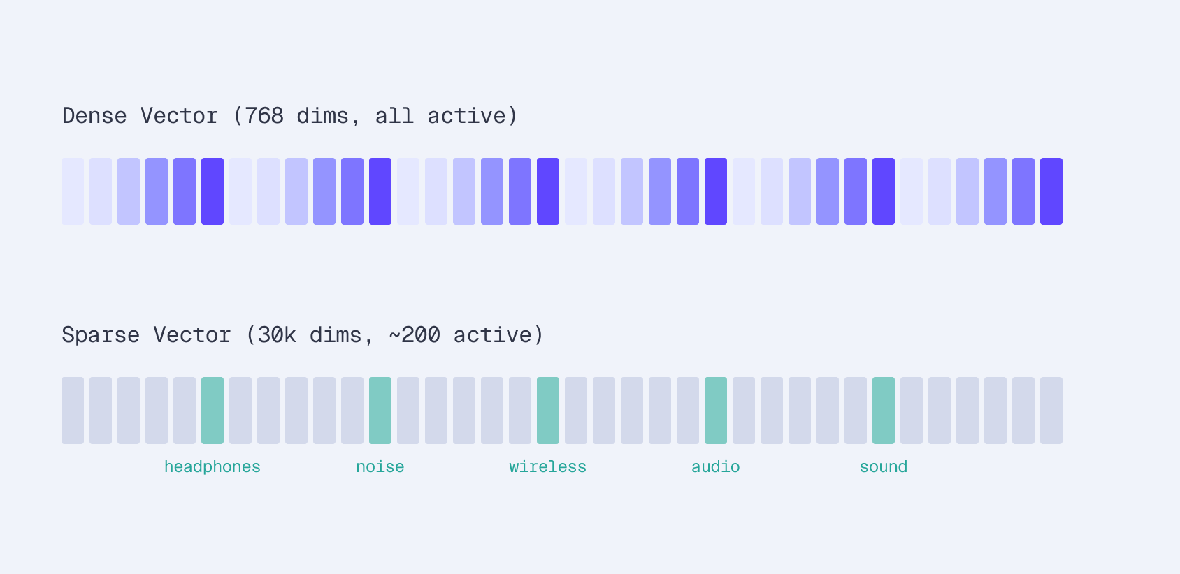
Both approaches encode text into vectors, but sparse embeddings preserve individual term signals that dense models compress away.
The key difference: each dimension in a sparse vector corresponds to an actual word in the vocabulary. You can inspect the vector and see exactly which terms the model considers important and how much weight it gives each one.
SPLADE: Learned Sparse Representations
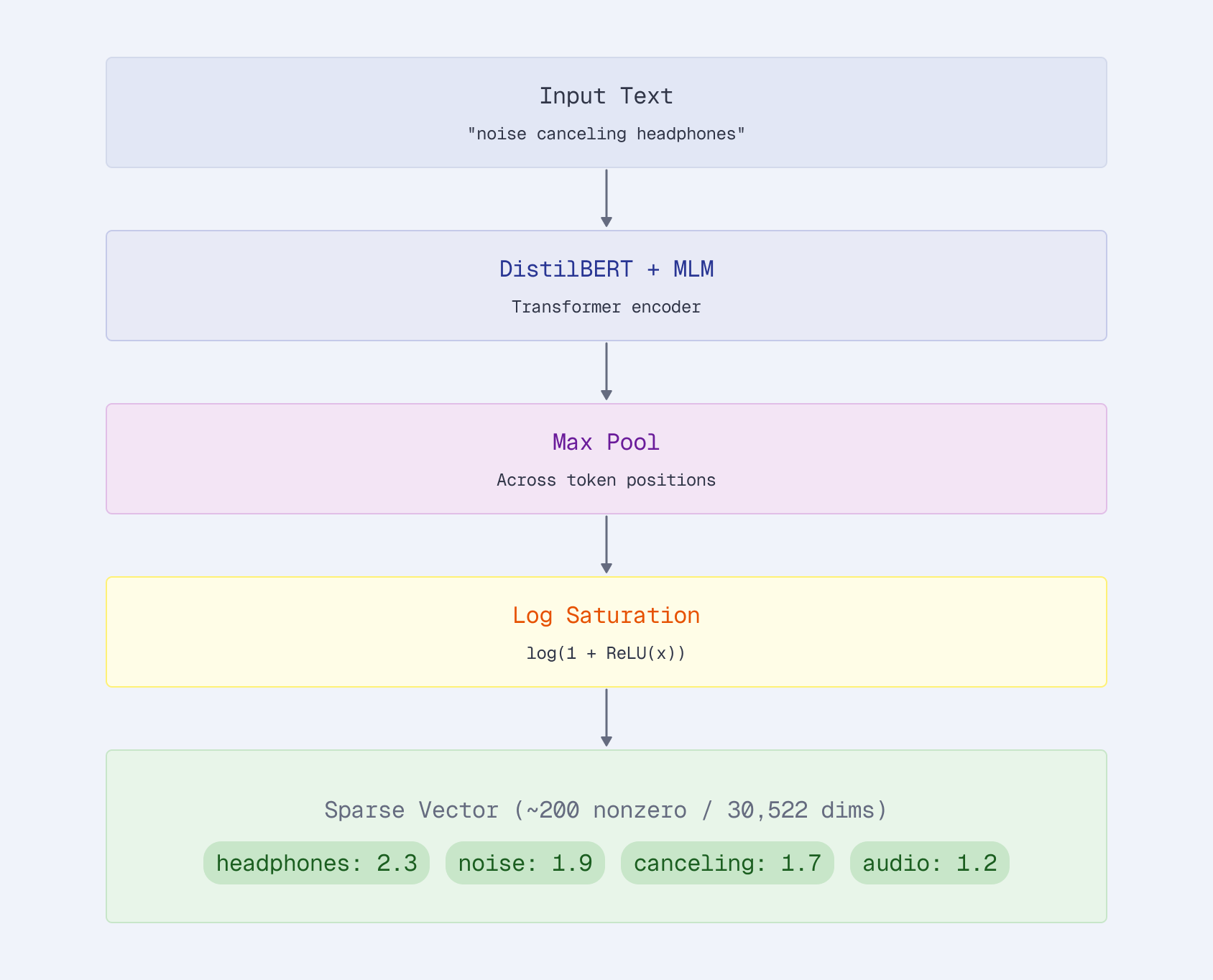
SPLADE (Sparse Lexical and Expansion) is the model architecture that makes this work. It passes text through a transformer with a masked language model (MLM) head, then applies max pooling and log saturation to produce sparse weights:
For an input like "noise canceling headphones", SPLADE encodes it in four steps:
- Tokenize and encode the input through DistilBERT with a masked language model (MLM) head
- Max pool across all token positions to get a single score per vocabulary term
- Apply log saturation —
log(1 + ReLU(x))— a learned version of BM25’s saturation curve that prevents any single term from dominating - Output a sparse vector with ~200 non-zero values out of 30,522 vocabulary dimensions
| Token | Weight |
|---|---|
| headphones | 2.3 |
| noise | 1.9 |
| canceling | 1.7 |
| audio | 1.2 |
| wireless | 0.8 |
| sound | 0.6 |
The log saturation step is important. Without it, a single high-confidence term could dominate the score. The log compression keeps results balanced - “headphones” matters more than “audio”, but not 10x more.
The model learns three things simultaneously:
- Weight important terms higher (product names, key attributes)
- Expand queries with related terms (implicit synonym expansion)
- Suppress noise (common words get near-zero weights)
Query Expansion: Why SPLADE Beats BM25
This expansion is what separates SPLADE from traditional keyword search. BM25 can only match terms that literally appear in both the query and the document. SPLADE adds related terms that the model learned from training data:
Query: “summer dress”
Original terms: dress (2.5), summer (2.1)
Expanded by SPLADE: sundress (1.8), floral (0.9), lightweight (0.7), cotton (0.6)
The model adds “sundress”, “floral”, and “cotton” - terms that appear in product titles even when “summer” doesn’t. This matches products like “Floral Sundress for Women - Lightweight Cotton” that BM25 would miss entirely.
No manual synonym file. No query rewriting rules. The model learned these associations from seeing millions of query-product pairs.
Why Qdrant for Sparse Vectors?
Not every vector database treats sparse vectors as a first-class citizen. Qdrant does, and the difference matters in practice.
Weighted sparse vectors. SPLADE emits arbitrary learned weights; Qdrant stores them natively. If you’re running a BM25 baseline, you can still add IDF at query time:
sparse_vectors_config={
    "bm25": models.SparseVectorParams(
        modifier=models.Modifier.IDF,  # Apply IDF at query time
    )
}
Hybrid in one request. Combine sparse precision with dense semantics via native RRF/prefetch - no external reranker:
client.query_points(
    collection_name="products",
    prefetch=[
        models.Prefetch(query=sparse_vector, using="sparse", limit=100),
        models.Prefetch(query=dense_vector, using="dense", limit=100),
    ],
    query=models.FusionQuery(fusion=models.Fusion.RRF),
    limit=10,
)
Production-ready scaling. Rust + SIMD-optimized inverted index with an on-disk option keeps RAM low even with 200+ active terms per doc across millions of products.
No ANN approximation. Sparse retrieval uses an inverted index, the same data structure powering BM25. Results are exact - no recall tradeoffs from approximate nearest neighbor search.
The Stack
Our training pipeline combines three components:
Modal (GPU Training)
- A100 GPUs on demand
- Persistent volumes for checkpoints
- Detached runs for long training
Sentence Transformers v5 (Training Framework)
- SparseEncoder architecture
- SpladeLoss with regularization
- Built-in training utilities
Qdrant (Sparse Vector Store)
- Native sparse vector support
- Inverted index
- Hybrid search ready
Modal gives us serverless A100 GPUs - no idle hardware, no queue management. Sentence Transformers v5 introduced the SparseEncoder class that makes SPLADE training straightforward. And Qdrant handles storage, indexing, and retrieval with native sparse vector support.
What We’ll Build
Over the next four articles, we’ll walk through the full pipeline:
Part 2: Training on Modal - Loading the Amazon ESCI dataset, creating the SPLADE model, configuring loss functions with sparsity regularization, and running GPU training with persistent checkpoints.
Part 3: Evaluation and Hard Negative Mining - Indexing products in Qdrant, running retrieval benchmarks (nDCG, MRR, Recall), implementing ANCE hard negative mining loops, and analyzing what fine-tuning actually changes in the model.
Part 4: Specialization vs Generalization - Cross-domain evaluation on Wayfair and Home Depot data, multi-domain training, when to specialize vs generalize, and production deployment guidance.
Part 5: From Research to Product - An open-source CLI and web dashboard that runs the entire fine-tuning pipeline with a single command.
The end result: a fine-tuned SPLADE model that achieves nDCG@10 of 0.388 on Amazon ESCI, compared to 0.301 for BM25 and 0.324 for off-the-shelf SPLADE. That 29% improvement over BM25 translates to meaningfully better search results for real e-commerce queries. You can try the models directly from HuggingFace: splade-ecommerce-esci (best in-domain) and splade-ecommerce-multidomain (better generalization).