Fine-Tuning Sparse Embeddings for E-Commerce Search | Part 3: Evaluation and Hard Negatives
Thierry Damiba
·March 09, 2026

This is Part 3 of a 5-part series on fine-tuning sparse embeddings for e-commerce search. In Part 2, we trained a SPLADE model on Modal. Now we evaluate it and push further with hard negative mining.
Series:
- Part 1: Why Sparse Embeddings Beat BM25
- Part 2: Training SPLADE on Modal
- Part 3: Evaluation & Hard Negatives (here)
- Part 4: Specialization vs Generalization
- Part 5: From Research to Product
We have a trained SPLADE model sitting on a Modal volume (or grab it from HuggingFace). Now comes the question that matters: is it actually better? In this article, we’ll index products into Qdrant, run retrieval benchmarks, implement hard negative mining, and dig into what the model learned. Full evaluation code is in the GitHub repo. To run this entire pipeline on your own data, see the sparse-finetune CLI.
Indexing Products in Qdrant
Before we can evaluate, we need products in a searchable index. Qdrant’s sparse vector support makes this straightforward:
from qdrant_client import QdrantClient, models

def index_products(model, products, collection_name="ecommerce_splade"):
    client = QdrantClient(url=QDRANT_URL, api_key=QDRANT_API_KEY)

    # Create collection with sparse vector config
    client.create_collection(
        collection_name=collection_name,
        vectors_config={},
        sparse_vectors_config={
            "text": models.SparseVectorParams(
                index=models.SparseIndexParams(on_disk=True)
            )
        },
    )

    # Encode and index in batches
    for batch in chunked(products, batch_size=32):
        texts = [p["text"] for p in batch]
        embeddings = model.encode(texts)

        points = []
        for product, emb in zip(batch, embeddings):
            indices = emb["indices"].tolist()
            values = emb["values"].tolist()

            points.append(models.PointStruct(
                id=product["id"],
                vector={
                    "text": models.SparseVector(indices=indices, values=values)
                },
                payload={"title": product["title"], "brand": product["brand"]},
            ))

        upsert_with_retry(client, collection_name, points)
A few production details:
on_disk=Truekeeps the inverted index on disk instead of RAM. SPLADE vectors average 200 active terms, and across millions of products, this adds up. Requires SSD for acceptable latency.wait=Falseon upserts (insideupsert_with_retry) lets you pipeline batches without blocking. Call withwait=Trueon the final batch.- Retry with exponential backoff for cloud databases. Network hiccups happen in production.
def upsert_with_retry(client, collection_name, points, max_retries=5):
    """Upsert with exponential backoff."""
    for attempt in range(max_retries):
        try:
            client.upsert(collection_name=collection_name, points=points, wait=False)
            return
        except Exception as e:
            if attempt == max_retries - 1:
                raise
            wait_time = (2 ** attempt) + (attempt * 0.5)
            time.sleep(wait_time)
Retrieval Metrics
We evaluate with standard information retrieval metrics on 2,000 test queries against 10,000 products:
- nDCG@k — Ranking quality with position bias; top results matter more
- MRR@k — How high the first relevant result appears
- Recall@k — What fraction of relevant products appear in top-k
- Precision@k — What fraction of top-k results are relevant
nDCG@10 (Normalized Discounted Cumulative Gain) is the primary metric. It rewards putting highly relevant products (Exact matches) at the top and penalizes relevant results that appear lower in the ranking. A perfect score is 1.0; random ranking on this dataset gives roughly 0.1.
Searching the Index
def search_products(query, model, client, collection_name="ecommerce_splade", limit=10):
    query_embedding = model.encode(query)

    results = client.query_points(
        collection_name=collection_name,
        query=models.SparseVector(
            indices=query_embedding["indices"].tolist(),
            values=query_embedding["values"].tolist(),
        ),
        using="text",
        limit=limit,
    )

    return [
        {"id": r.id, "score": r.score, "title": r.payload["title"]}
        for r in results.points
    ]
Five lines from query string to ranked products. The sparse vector lookup in Qdrant’s inverted index is sub-millisecond, even with millions of products. The bottleneck is the 10-20ms query encoding through the transformer.
The Results
Here’s what we found, evaluated on 2,000 test queries:
| Model | nDCG@10 | MRR@10 | vs BM25 |
|---|---|---|---|
| BM25 (baseline) | 0.305 | 0.313 | - |
| SPLADE (off-the-shelf) | 0.326 | 0.339 | +7.2% |
| SPLADE (fine-tuned) | 0.389 | 0.387 | +27.5% |
The fine-tuned model beats BM25 by nearly 28%. More telling: it beats the off-the-shelf SPLADE by 19%. The off-the-shelf model was trained on MS MARCO (web search queries), not e-commerce. That 19% gap is the value of domain-specific training.
What About Hybrid Search?
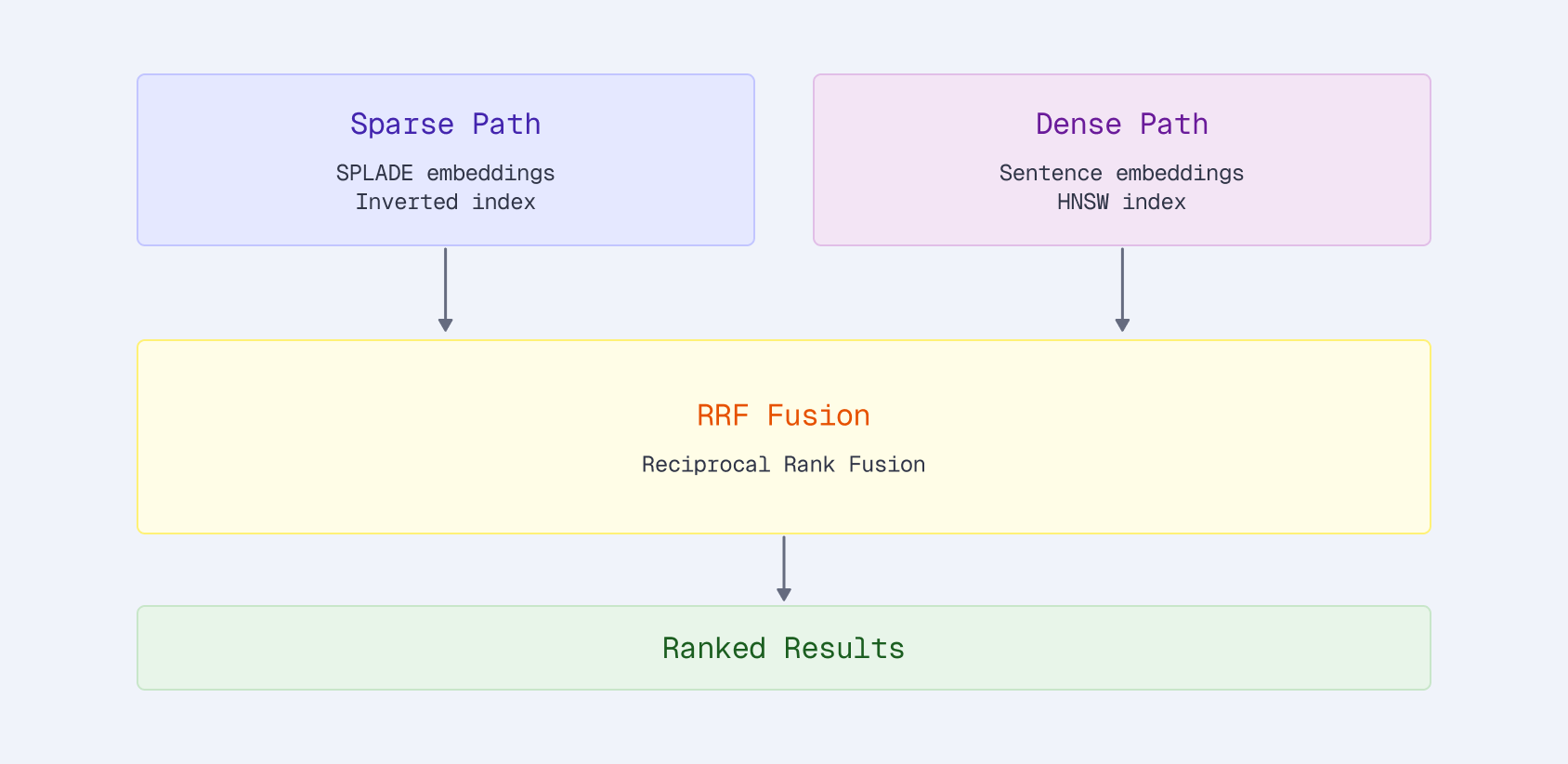
A natural question: can we combine sparse and dense vectors for even better results? We tested this with Qdrant’s native Reciprocal Rank Fusion:
client.query_points(
    collection_name="products",
    prefetch=[
        models.Prefetch(query=sparse_vector, using="sparse", limit=100),
        models.Prefetch(query=dense_vector, using="dense", limit=100),
    ],
    query=models.FusionQuery(fusion=models.Fusion.RRF),
    limit=10,
)
With the off-the-shelf SPLADE, hybrid helps: +1.3% over sparse alone. Both signals are moderate strength, and combining them catches products that either one misses.
With the fine-tuned SPLADE, hybrid actually hurts: SPLADE-only scored 0.413 vs hybrid at 0.405. The fine-tuned sparse model is strong enough that adding a generic dense signal dilutes the ranking. The dense model retrieves semantically similar but irrelevant products that drag down nDCG.
This is a useful finding. Hybrid search isn’t always better. It depends on the relative strength of your signals. If your sparse model is domain-tuned and your dense model is generic, the dense component can actively harm results.
Hard Negative Mining with ANCE
The training in Part 2 used in-batch negatives: other products in the same batch serve as negatives for a given query. This works but has a limitation: random products are easy negatives. The model doesn’t learn to distinguish between genuinely confusable products.
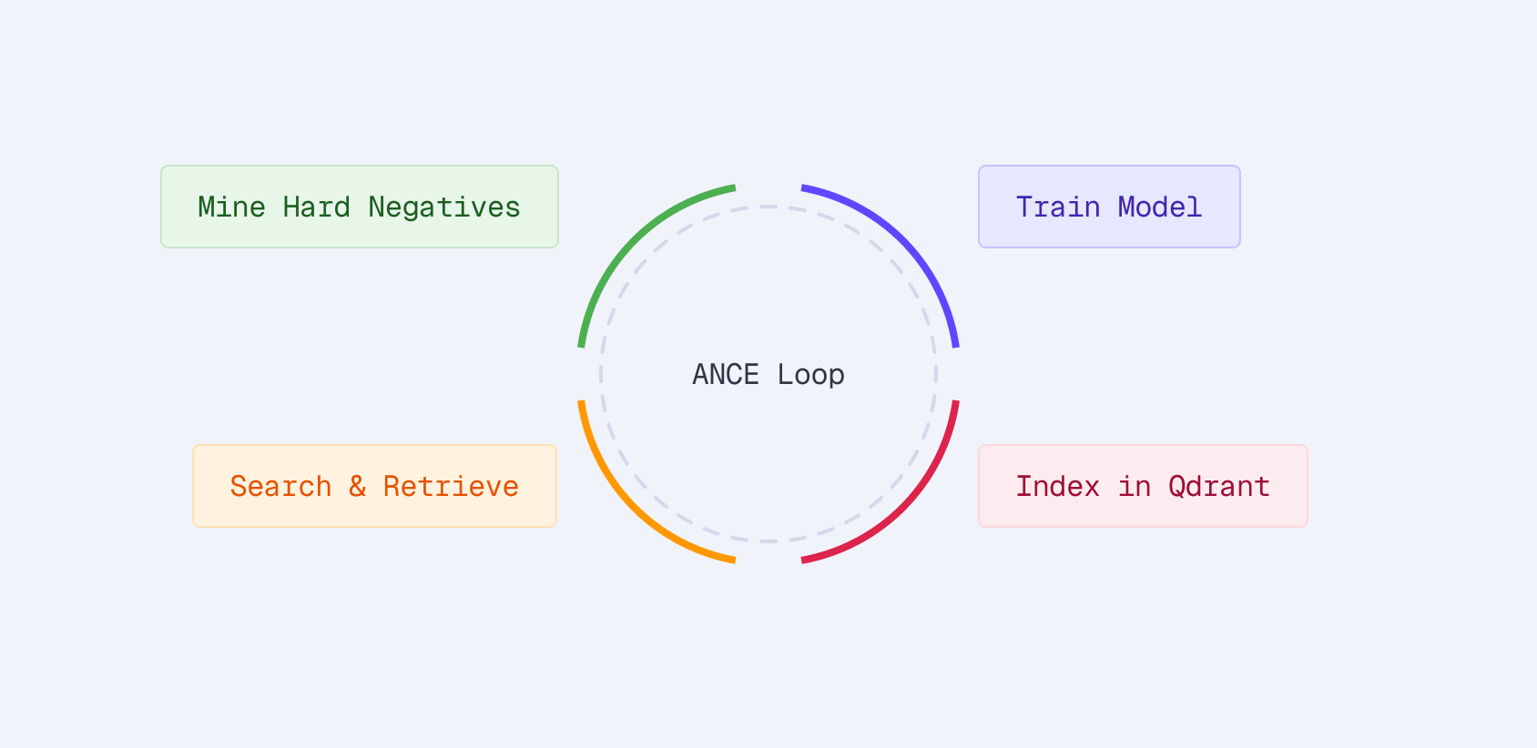
ANCE (Approximate Nearest Neighbor Negative Contrastive Estimation) fixes this by mining hard negatives from the current model’s own retrieval results:
- Index products into Qdrant with the current model
- Retrieve top-K products for each query
- Filter to non-relevant products — these are the hard negatives
- Train on (query, positive, hard_negatives) triplets
- Repeat with the updated model
Each round mines harder negatives as the model improves.
The idea: if the current model retrieves a product for a query but that product isn’t relevant, it’s a hard negative. The model thought it was relevant, so training on it teaches the model where its mistakes are.
Mining Implementation
from src.qdrant.mining import SparseQdrantMiner

# Index products with current model
index_sparse_vectors(client, collection_name, model, products)

# Mine hard negatives
miner = SparseQdrantMiner(client, model, collection_name)
hard_neg_examples = miner.mine_for_training(
    queries=queries_with_positives,
    top_k=20,           # Consider top-20 results
    num_negatives=3,    # Keep 3 hardest negatives per query
)

# hard_neg_examples now contains:
# [{"anchor": "wireless earbuds",
#   "positive": "Sony WF-1000XM5 Earbuds...",
#   "negative": ["Generic Bluetooth Earbuds...", ...]}, ...]
Sparse retrieval keeps mining cheap, with sub-millisecond per query in Qdrant. For 100K queries, the mining step takes seconds, not minutes. Payload filters exclude known positives so you don’t accidentally treat a relevant product as a negative.
When to Use ANCE
ANCE adds complexity. You need to:
- Index products with the current model
- Run retrieval for all training queries
- Filter and format the results
- Retrain with the augmented dataset
- Optionally repeat
This gives an additional 5-10% improvement on top of basic training. Whether that’s worth the engineering effort depends on your use case. For a product search system serving millions of queries, 5% nDCG improvement translates to meaningfully better user experience and conversion rates.
What Fine-Tuning Actually Changes
Looking at the model’s outputs before and after fine-tuning reveals what it learned:
Query expansion improves:
- “laptop” → adds “notebook”, “computer”, “macbook”
- “wireless earbuds” → adds “bluetooth”, “airpods”, “tws”
Term weighting sharpens:
- Brand names get higher weights (users searching “Sony headphones” want Sony)
- Generic terms get lower weights (“good”, “best”, “cheap”)
Domain vocabulary emerges:
- E-commerce terms like “refurbished”, “renewed”, “bundle” get meaningful weights
- Web-search-specific terms get downweighted
This domain adaptation explains both the strong in-domain results and, as we’ll see in Part 4, the tradeoffs when applying the model to other domains.
Production Latency
A common concern: isn’t running a transformer on every query slow?
| Step | Latency | Note |
|---|---|---|
| Query encoding (SPLADE) | 10-20ms | Bottleneck |
| Sparse retrieval (Qdrant) | <1ms | Negligible |
| Total | 10-20ms | Real-time |
The retrieval itself is negligible. Qdrant’s Rust + SIMD-optimized inverted index scans millions of posting lists in sub-millisecond time. All the latency is in the encoder, which runs once per query regardless of catalog size.
Optimization strategies if 15ms isn’t fast enough:
- Batch queries: Encode multiple queries together (autocomplete, related searches)
- Distillation: Train a smaller encoder (TinyBERT, MiniLM) to mimic SPLADE’s outputs
- Caching: Popular queries can be cached at the sparse vector level
- GPU inference: 5-10x speedup on high-traffic systems
For most e-commerce applications, 15ms is fine, especially when it delivers 28% better relevance.
Key Takeaways
- Fine-tuned SPLADE beats BM25 by 28% and off-the-shelf SPLADE by 19%. Domain-specific training matters, even for sparse models.
- Hybrid search isn’t always better. A strong domain-tuned sparse model can outperform sparse+dense fusion when the dense component is generic.
- Hard negative mining (ANCE) adds 5-10% on top of basic training. Qdrant’s sparse retrieval makes the mining step cheap.
- Production latency is 10-20ms total. Transformer encoding is the bottleneck, not retrieval.
- The model learns domain-specific patterns: query expansion, term weighting, and e-commerce vocabulary all improve with fine-tuning.