Combining Vector Search and Filtering
We’ve talked about how Qdrant uses the HNSW graph to efficiently search dense vectors. But in real-world applications, you’ll often want to constrain your search using filters. This creates unique challenges for graph traversal that Qdrant solves elegantly.
The Challenge: Filters Break Graph Connectivity
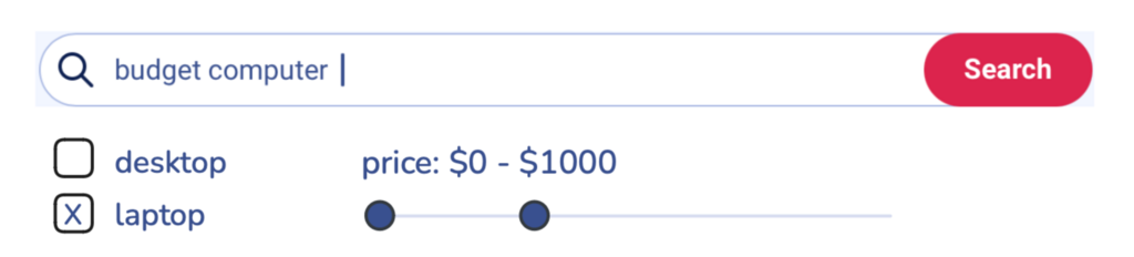
Consider retrieving items from an online store collection where you only want to show laptops priced under $1,000. That price information, along with the category ’laptop’, isn’t part of the vector - it lives in the payload.
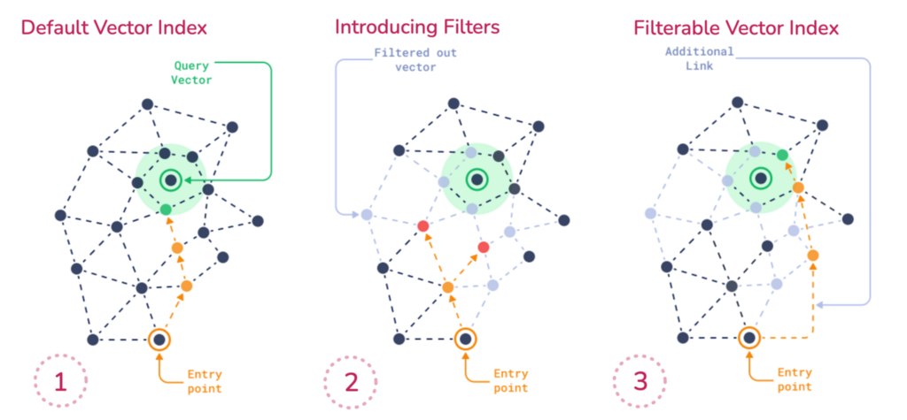
When you apply a filter like price < 1000, you’re essentially restricting which points are eligible during search. This introduces challenges for graph traversal because HNSW depends on both short- and long-range edges to efficiently explore the vector space. It requires any point in the graph to be reachable. But if filtering removes a large portion of those points, the search path can break. You risk missing relevant results - not because they weren’t similar, but because they were unreachable under the filter.
Naive Approaches and Their Problems
Post-Filtering
One approach is to ignore the filter initially: run the search across the whole dataset, get the top K most similar vectors, then apply the filter afterward.
The problem: You might discard most of the top K results. If the best match that satisfies the filter wasn’t in that top K, you won’t retrieve it. You waste compute and lose recall because relevant points were never retrieved.
Pre-filtering
Another approach is to filter first, Then search inside the filtered set.
The problem: When filters are too restrictive, they fragment the HNSW graph, breaking connectivity and making traversal inefficient or impossible.
Qdrant’s Solution: Filterable HNSW
Qdrant solves this with a smarter approach. We guarantee that the HNSW graph remains connected by creating additional edges to maintain connectivity under filtering. Qdrant builds subgraphs per payload value, then merges them back into the full graph.
So if you filter brand = Apple, Qdrant has already built a connected subgraph of just Apple points, and traversal works fine within that subset.
The Query Planner: Adaptive Strategy
At query time, Qdrant uses a query planner to determine the appropriate strategy. This planning happens per segment and is based on filter cardinality, index availability, and thresholds like full_scan_threshold.
- Filter matches many points: Qdrant performs regular HNSW search but skips over nodes that don’t match during traversal. This avoids the cost of pre-filtering a large result set while keeping the search fast and approximate.
- Filter matches few points: If the filter matches just a tiny portion of the collection, Qdrant might skip HNSW entirely and fall back to a simple full scan if that’s faster.
Payload Indexing: The Base Layer
Critical point: Qdrant does not index payload fields by default. You must explicitly define which fields to index. Best practice is to create payload indexes before uploading any data so HNSW can build filter-aware links. If you add payload indexes after HNSW was built, searches may run less efficiently until you rebuild. To rebuild, change m to recreate HNSW per segment but bear in mind that rebuilding is compute heavy on large collections.
from qdrant_client import QdrantClient, models
import os

client = QdrantClient(url=os.getenv("QDRANT_URL"), api_key=os.getenv("QDRANT_API_KEY"))

# For Colab:
# from google.colab import userdata
# client = QdrantClient(url=userdata.get("QDRANT_URL"), api_key=userdata.get("QDRANT_API_KEY"))

collection_name = "store"
vector_size = 768

if client.collection_exists(collection_name=collection_name):
    client.delete_collection(collection_name=collection_name)

client.create_collection(
    collection_name=collection_name,
    vectors_config=models.VectorParams(
        size=vector_size,
        distance=models.Distance.COSINE,
    ),
    optimizers_config=models.OptimizersConfigDiff(
        indexing_threshold=100,
    ),
)

# Index frequently filtered fields
client.create_payload_index(
    collection_name=collection_name,
    field_name="category",
    field_schema=models.PayloadSchemaType.KEYWORD,
)

client.create_payload_index(
    collection_name=collection_name,
    field_name="price",
    field_schema=models.PayloadSchemaType.FLOAT,
)

client.create_payload_index(
    collection_name=collection_name,
    field_name="brand",
    field_schema=models.PayloadSchemaType.KEYWORD,
)
Add sample data:
# Upload data
import random

points = []
for i in range(1000):
    points.append(
        models.PointStruct(
            id=i,
            vector=[random.random() for _ in range(vector_size)],
            payload={
                "category": random.choice(["laptop", "phone", "tablet"]),
                "price": random.randint(0, 1000),
                "brand": random.choice(
                    ["Apple", "Dell", "HP", "Lenovo", "Asus", "Acer", "Samsung"]
                ),
            },
        )
    )
client.upload_points(
    collection_name=collection_name,
    points=points,
)
Memory Considerations
Payload indexes consume additional memory, so it’s recommended to only index fields used in filtering conditions.
If memory is limited, prioritise the field that produces the most specific search results. The more varied and granular the payload field values are, the more effective it’s index will be.
Practical Implementation
Setting Up Filterable Search
The following example illustrates how filtering is carried out in practice:
# Create filter combining multiple conditions
filter_conditions = models.Filter(
    must=[
        models.FieldCondition(key="category", match=models.MatchValue(value="laptop")),
        models.FieldCondition(key="price", range=models.Range(lte=1000)),
        models.FieldCondition(key="brand", match=models.MatchAny(any=["Apple", "Dell", "HP"])),
    ]
)

query_vector = [random.random() for _ in range(vector_size)]

# Execute filtered search
results = client.query_points(
    collection_name=collection_name,
    query=query_vector,
    query_filter=filter_conditions,
    limit=10,
    search_params=models.SearchParams(hnsw_ef=128),
)
See more in the docs.
Query Planner Decision Matrix
| Filter Cardinality | Strategy | When Used |
|---|---|---|
| High (many matches) | HNSW with node skipping | Filter matches many points |
| Very low (few matches) | Full scan over candidates | Tiny result set |
Performance Optimization Tips
- Index early: Create payload indexes before HNSW build.
- Index the right fields: Create payload indexes for all filtered fields. Prefer high-selectivity fields if memory is limited.
- Test filter combinations: Complex multi-field filters gain the most from proper indexing.
- Tune thresholds: Adjust
full_scan_thresholdbased on your data distribution and query patterns - Measure real performance: Benchmark with your actual data and query patterns to validate planner decisions
Key Takeaways
Filterable HNSW is not a separate indexing mechanism, it extends the HNSW graph by adding extra edges based on stored payload values to maintain traversal performance under filtering constraints.
The query planner automatically selects the optimal strategy based on filter selectivity, available indexes, and segment characteristics.
Payload indexing is essential for filtered search performance, especially with large datasets and complex filter conditions.
Always benchmark with your specific data to understand how the planner behaves and optimize accordingly.
In the next section, we’ll define a collection with structured payloads, configure payload indexing, and evaluate how different HNSW parameters impact filtered search performance.
Learn more: Filterable HNSW Article