Vector Search Resource Optimization Guide
David Myriel
·February 09, 2025

What’s in This Guide?
Resource Management Strategies: If you are trying to scale your app on a budget - this is the guide for you. We will show you how to avoid wasting compute resources and get the maximum return on your investment.
Performance Improvement Tricks: We’ll dive into advanced techniques like indexing, compression, and partitioning. Our tips will help you get better results at scale, while reducing total resource expenditure.
Query Optimization Methods: Improving your vector database setup isn’t just about saving costs. We’ll show you how to build search systems that deliver consistently high precision while staying adaptable.
Remember: Optimization is a Balancing Act
In this guide, we will show you how to use Qdrant’s features to meet your performance needs. However - there are resource tradeoffs and you can’t have it all. It is up to you to choose the optimization strategy that best fits your goals.
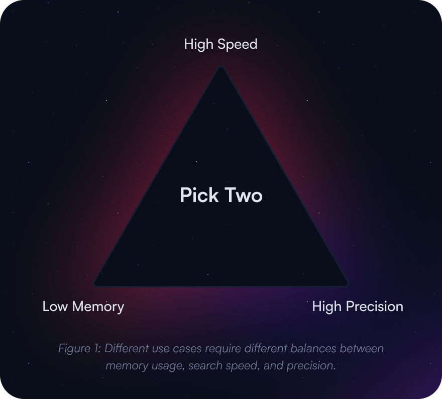
Let’s take a look at some common goals and optimization strategies:
After this article, check out the code samples in our docs on Qdrant’s Optimization Methods.
Configure Indexing for Faster Searches

A vector index is the central location where Qdrant calculates vector similarity. It is the backbone of your search process, retrieving relevant results from vast amounts of data.
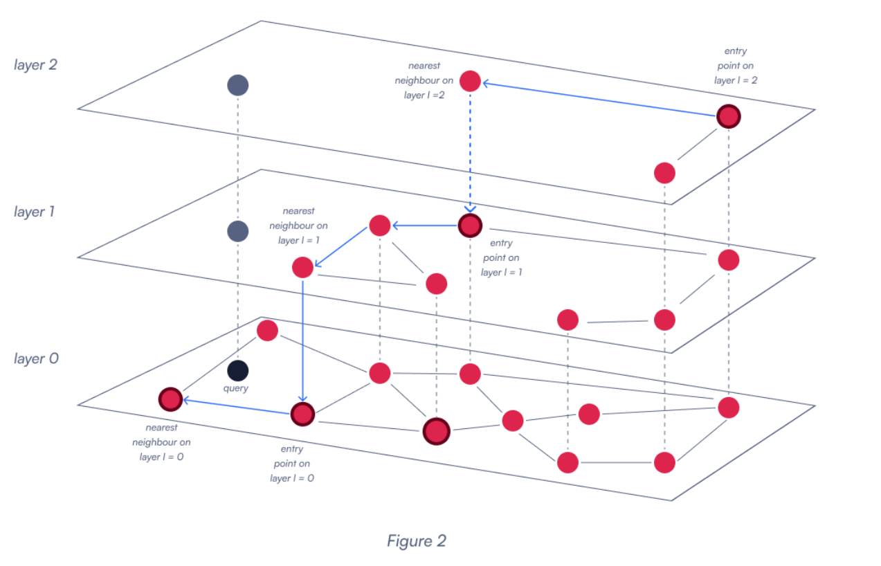
Qdrant uses the HNSW (Hierarchical Navigable Small World Graph) algorithm as its dense vector index, which is both powerful and scalable.
Figure 2: A sample HNSW vector index with three layers. Follow the blue arrow on the top layer to see how a query travels throughout the database index. The closest result is on the bottom level, nearest to the gray query point.
Vector Index Optimization Parameters
Working with massive datasets that contain billions of vectors demands significant resources—and those resources come with a price. While Qdrant provides reasonable defaults, tailoring them to your specific use case can unlock optimal performance. Here’s what you need to know.
The following parameters give you the flexibility to fine-tune Qdrant’s performance for your specific workload. You can modify them directly in Qdrant’s configuration files or at the collection and named vector levels for more granular control.
Figure 3: A description of three key HNSW parameters.
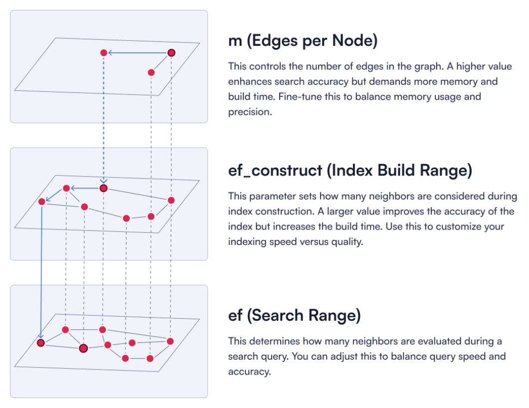
1. The m parameter determines edges per node
This controls the number of edges in the graph. A higher value enhances search accuracy but demands more memory and build time. Fine-tune this to balance memory usage and precision.
2. The ef_construct parameter controls the index build range
This parameter sets how many neighbors are considered during index construction. A larger value improves the accuracy of the index but increases the build time. Use this to customize your indexing speed versus quality.
You need to set both the m and ef parameters as you create the collection:
client.update_collection(
    collection_name="{collection_name}",
    vectors_config={
        "my_vector": models.VectorParamsDiff(
            hnsw_config=models.HnswConfigDiff(
                m=32,
                ef_construct=123,
            ),
        ),
    }
)
3. The ef parameter updates vector search range
This determines how many neighbors are evaluated during a search query. You can adjust this to balance query speed and accuracy.
The ef parameter is configured during the search process:
client.query_points(
   collection_name="{collection_name}",
   query=[...]
   search_params=models.SearchParams(hnsw_ef=128, exact=False),
)
These are just the basics of HNSW. Learn More about Indexing.
Data Compression Techniques

Efficient data compression is a cornerstone of resource optimization in vector databases. By reducing memory usage, you can achieve faster query performance without sacrificing too much accuracy.
One powerful technique is quantization, which transforms high-dimensional vectors into compact representations while preserving relative similarity. Let’s explore the quantization options available in Qdrant.
Scalar Quantization
Scalar quantization strikes an excellent balance between compression and performance, making it the go-to choice for most use cases.
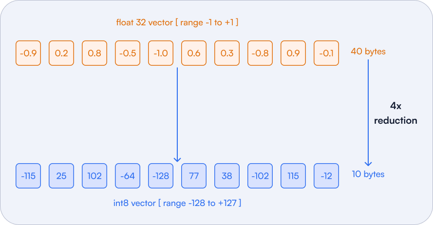
This method minimizes the number of bits used to represent each vector component. For instance, Qdrant compresses 32-bit floating-point values (float32) into 8-bit unsigned integers (uint8), slashing memory usage by an impressive 75%.
Figure 4: The top example shows a float32 vector with a size of 40 bytes. Converting it to int8 format reduces its size by a factor of four, while maintaining approximate similarity relationships between vectors. The loss in precision compared to the original representation is typically negligible for most practical applications.
Benefits of Scalar Quantization:
| Benefit | Description |
|---|---|
| Memory usage will drop | Compression cuts memory usage by a factor of 4. Qdrant compresses 32-bit floating-point values (float32) into 8-bit unsigned integers (uint8). |
| Accuracy loss is minimal | Converting from float32 to uint8 introduces a small loss in precision. Typical error rates remain below 1%, making this method highly efficient. |
| Best for specific use cases | To be used with high-dimensional vectors where minor accuracy losses are acceptable. |
Set it up as you create the collection:
client.create_collection(
   collection_name="{collection_name}",
   vectors_config=models.VectorParams(size=1536, distance=models.Distance.COSINE),
   quantization_config=models.ScalarQuantization(
       scalar=models.ScalarQuantizationConfig(
           type=models.ScalarType.INT8,
           quantile=0.99,
           always_ram=True,
       ),
   ),
)
When working with Qdrant, you can fine-tune the quantization configuration to optimize precision, memory usage, and performance. Here’s what the key configuration options include:
| Configuration Option | Description |
|---|---|
type | Specifies the quantized vector type (currently supports only int8). |
quantile | Sets bounds for quantization, excluding outliers. For example, 0.99 excludes the top 1% of extreme values to maintain better accuracy. |
always_ram | Keeps quantized vectors in RAM to speed up searches. |
Adjust these settings to strike the right balance between precision and efficiency for your specific workload.
Learn More about Scalar Quantization
Binary Quantization
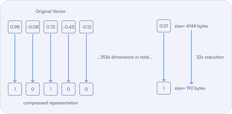
Binary quantization takes scalar quantization to the next level by compressing each vector component into just a single bit. This method achieves unparalleled memory efficiency and query speed, reducing memory usage by a factor of 32 and enabling searches up to 40x faster.
Benefits of Binary Quantization:
Binary quantization is ideal for large-scale datasets and compatible embedding models, where compression and speed are paramount.
Figure 5: This method causes maximum compression. It reduces memory usage by 32x and speeds up searches by up to 40x.
| Benefit | Description |
|---|---|
| Efficient similarity calculations | Emulates Hamming distance through dot product comparisons, making it fast and effective. |
| Perfect for high-dimensional vectors | Works well with embedding models like OpenAI’s text-embedding-ada-002 or Cohere’s embed-english-v3.0. |
| Precision management | Consider rescoring or oversampling to offset precision loss. |
Here’s how you can enable binary quantization in Qdrant:
client.create_collection(
   collection_name="{collection_name}",
   vectors_config=models.VectorParams(size=1536, distance=models.Distance.COSINE),
   quantization_config=models.BinaryQuantization(
       binary=models.BinaryQuantizationConfig(
           always_ram=True,
       ),
   ),
)
By default, quantized vectors load like original vectors unless you set
always_ramtoTruefor instant access and faster queries.
Learn more about Binary Quantization
Scaling the Database

Efficiently managing large datasets in distributed systems like Qdrant requires smart strategies for data isolation. Multitenancy and Sharding are essential tools to help you handle high volumes of user-specific data while maintaining performance and scalability.
Multitenancy
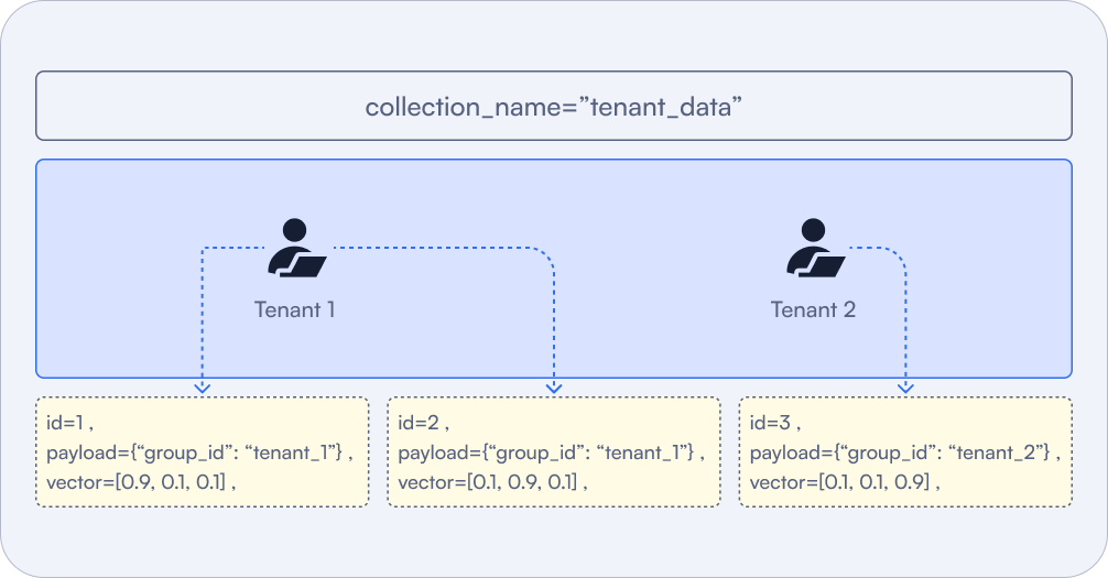
Multitenancy is a software architecture where multiple independent users (or tenants) share the same resources or environment. In Qdrant, a single collection with logical partitioning is often the most efficient setup for multitenant use cases.
Figure 5: Each individual vector is assigned a specific payload that denotes which tenant it belongs to. This is how a large number of different tenants can share a single Qdrant collection.
Why Choose Multitenancy?
- Logical Isolation: Ensures each tenant’s data remains separate while residing in the same collection.
- Minimized Overhead: Reduces resource consumption compared to maintaining separate collections for each user.
- Scalability: Handles high user volumes without compromising performance.
Here’s how you can implement multitenancy efficiently in Qdrant:
client.create_payload_index(
    collection_name="{collection_name}",
    field_name="group_id",
    field_schema=models.KeywordIndexParams(
        type="keyword",
        is_tenant=True,
    ),
)
Creating a keyword payload index, with the is_tenant parameter set to True, modifies the way the vectors will be logically stored. Storage structure will be organized to co-locate vectors of the same tenant together.
Now, each point stored in Qdrant should have the group_id payload attribute set:
client.upsert(
   collection_name="{collection_name}",
   points=[
       models.PointStruct(
           id=1,
           payload={"group_id": "user_1"},
           vector=[0.9, 0.1, 0.1],
       ),

       models.PointStruct(
           id=2,
           payload={"group_id": "user_2"},
           vector=[0.5, 0.9, 0.4],
       )
   ]
)
To ensure proper data isolation in a multitenant environment, you can assign a unique identifier, such as a group_id, to each vector. This approach ensures that each user’s data remains segregated, allowing users to access only their own data. You can further enhance this setup by applying filters during queries to restrict access to the relevant data.
Learn More about Multitenancy
Sharding
Sharding is a critical strategy in Qdrant for splitting collections into smaller units, called shards, to efficiently distribute data across multiple nodes. It’s a powerful tool for improving scalability and maintaining performance in large-scale systems.
User-Defined Sharding:
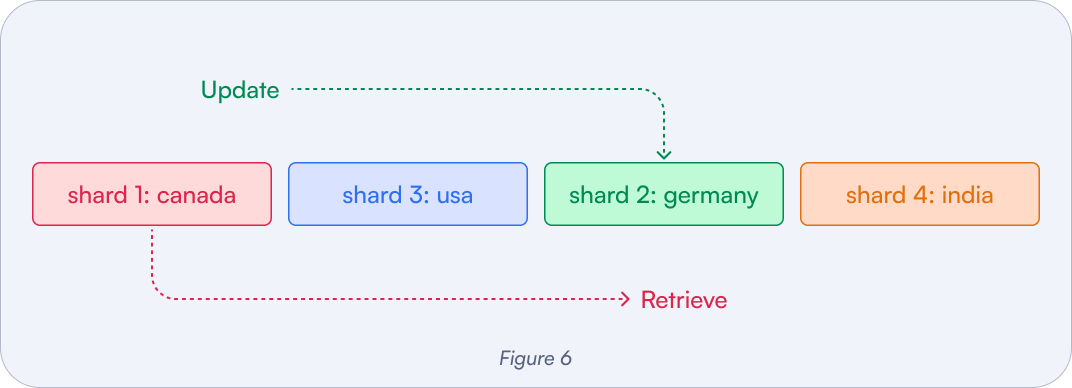
User-Defined Sharding allows you to take control of data placement by specifying a shard key. This feature is particularly useful in multi-tenant setups, as it enables the isolation of each tenant’s data within separate shards, ensuring better organization and enhanced data security.
Figure 6: Users can both upsert and query shards that are relevant to them, all within the same collection. Regional sharding can help avoid cross-continental traffic.
Example:
client.create_collection(
    collection_name="my_custom_sharded_collection",
    shard_number=1,
    sharding_method=models.ShardingMethod.CUSTOM
)
client.create_shard_key("my_custom_sharded_collection", "tenant_id")
When implementing user-defined sharding in Qdrant, two key parameters are critical to achieving efficient data distribution:
Shard Key:
The shard key determines how data points are distributed across shards. For example, using a key like
tenant_idallows you to control how Qdrant partitions the data. Each data point added to the collection will be assigned to a shard based on the value of this key, ensuring logical isolation of data.Shard Number:
This defines the total number of physical shards for each shard key, influencing resource allocation and query performance.
Here’s how you can add a data point to a collection with user-defined sharding:
client.upsert(
    collection_name="my_custom_sharded_collection",
    points=[
        models.PointStruct(
            id=1111,
            vector=[0.1, 0.2, 0.3]
        )
    ],
    shard_key_selector="tenant_1"
)
This code assigns the point to a specific shard based on the tenant_1 shard key, ensuring proper data placement.
Here’s how to choose the shard_number:
| Recommendation | Description |
|---|---|
| Match Shards to Nodes | The number of shards should align with the number of nodes in your cluster to balance resource utilization and query performance. |
| Plan for Scalability | Start with at least 2 shards per node to allow room for future growth. |
| Future-Proofing | Starting with around 12 shards is a good rule of thumb. This setup allows your system to scale seamlessly from 1 to 12 nodes without requiring re-sharding. |
Learn more about Sharding in Distributed Deployment
Query Optimization
 Improving vector database performance is critical when dealing with large datasets and complex queries. By leveraging techniques like filtering, batch processing, reranking, rescoring, and oversampling, so you can ensure fast response times and maintain efficiency even at scale.
Filtering
Filtering allows you to select only the required fields in your query results. By limiting the output size, you can significantly reduce response time and improve performance.
The filterable vector index is Qdrant’s solves pre and post-filtering problems by adding specialized links to the search graph. It aims to maintain the speed advantages of vector search while allowing for precise filtering, addressing the inefficiencies that can occur when applying filters after the vector search.
Example:
results = client.search(
    collection_name="my_collection",
    query_vector=[0.1, 0.2, 0.3],
    query_filter=models.Filter(must=[
        models.FieldCondition(
            key="category",
            match=models.MatchValue(value="my-category-name"),
        )
    ]),
    limit=10,
)
Figure 7: The filterable vector index adds specialized links to the search graph to speed up traversal.
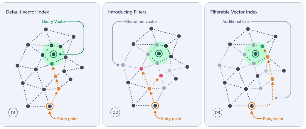
Filterable vector index: This technique builds additional links (orange) between leftover data points. The filtered points which stay behind are now traversible once again. Qdrant uses special category-based methods to connect these data points.
Read more about Filtering Docs and check out the Complete Filtering Guide.
Batch Processing
Batch processing consolidates multiple operations into a single execution cycle, reducing request overhead and enhancing throughput. It’s an effective strategy for both data insertion and query execution.
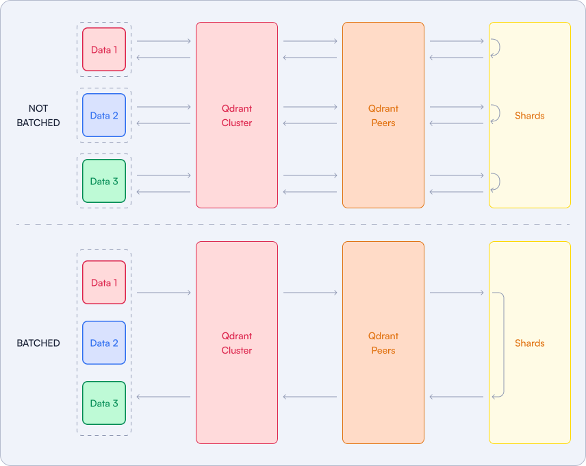
Batch Insertions: Instead of inserting vectors individually, group them into medium-sized batches to minimize the number of database requests and the overhead of frequent writes.
Example:
vectors = [
   [.1, .0, .0, .0],
   [.0, .1, .0, .0],
   [.0, .0, .1, .0],
   [.0, .0, .0, .1],
   …
]
client.upload_collection(
   collection_name="test_collection",
   vectors=vectors,
)
This reduces write operations and ensures faster data ingestion.
Batch Queries: Similarly, you can batch multiple queries together rather than executing them one by one. This reduces the number of round trips to the database, optimizing performance and reducing latency.
Example:
results = client.search_batch(
   collection_name="test_collection",
   requests=[
       SearchRequest(
           vector=[0., 0., 2., 0.],
           limit=1,
       ),
       SearchRequest(
           vector=[0., 0., 0., 0.01],
           with_vector=True,
           limit=2,
       )
   ]
)
Batch queries are particularly useful when processing a large number of similar queries or when handling multiple user requests simultaneously.
Hybrid Search
Hybrid search combines keyword filtering with vector similarity search, enabling faster and more precise results. Keywords help narrow down the dataset quickly, while vector similarity ensures semantic accuracy. This search method combines dense and sparse vectors.
Hybrid search in Qdrant uses both fusion and reranking. The former is about combining the results from different search methods, based solely on the scores returned by each method. That usually involves some normalization, as the scores returned by different methods might be in different ranges.
Figure 8: Hybrid Search Architecture
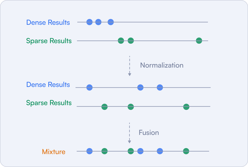
After that, there is a formula that takes the relevancy measures and calculates the final score that we use later on to reorder the documents. Qdrant has built-in support for the Reciprocal Rank Fusion method, which is the de facto standard in the field.
Learn more about Hybrid Search and read out Hybrid Queries docs.
Oversampling
Oversampling is a technique that helps compensate for any precision lost due to quantization. Since quantization simplifies vectors, some relevant matches could be missed in the initial search. To avoid this, you can retrieve more candidates, increasing the chances that the most relevant vectors make it into the final results.
You can control the number of extra candidates by setting an oversampling parameter. For example, if your desired number of results (limit) is 4 and you set an oversampling factor of 2, Qdrant will retrieve 8 candidates (4 × 2).
You can adjust the oversampling factor to control how many extra vectors Qdrant includes in the initial pool. More candidates mean a better chance of obtaining high-quality top-K results, especially after rescoring with the original vectors.
Learn more about Oversampling.
Rescoring
After oversampling to gather more potential matches, each candidate is re-evaluated based on additional criteria to ensure higher accuracy and relevance to the query.
The rescoring process maps the quantized vectors to their corresponding original vectors, allowing you to consider factors like context, metadata, or additional relevance that wasn’t included in the initial search, leading to more accurate results.
Example of Rescoring and Oversampling::
client.query_points(
    collection_name="my_collection",
    query_vector=[0.22, -0.01, -0.98, 0.37],
    search_params=models.SearchParams(
        quantization=models.QuantizationSearchParams(
            rescore=True,   # Enables rescoring with original vectors
            oversampling=2  # Retrieves extra candidates for rescoring
        )
    ),
    limit=4  # Desired number of final results
)
Learn more about Rescoring.
Reranking
Reranking adjusts the order of search results based on additional criteria, ensuring the most relevant results are prioritized.
This method is about taking the results from different search methods and reordering them based on some additional processing using the content of the documents, not just the scores. This processing may rely on an additional neural model, such as a cross-encoder which would be inefficient enough to be used on the whole dataset.
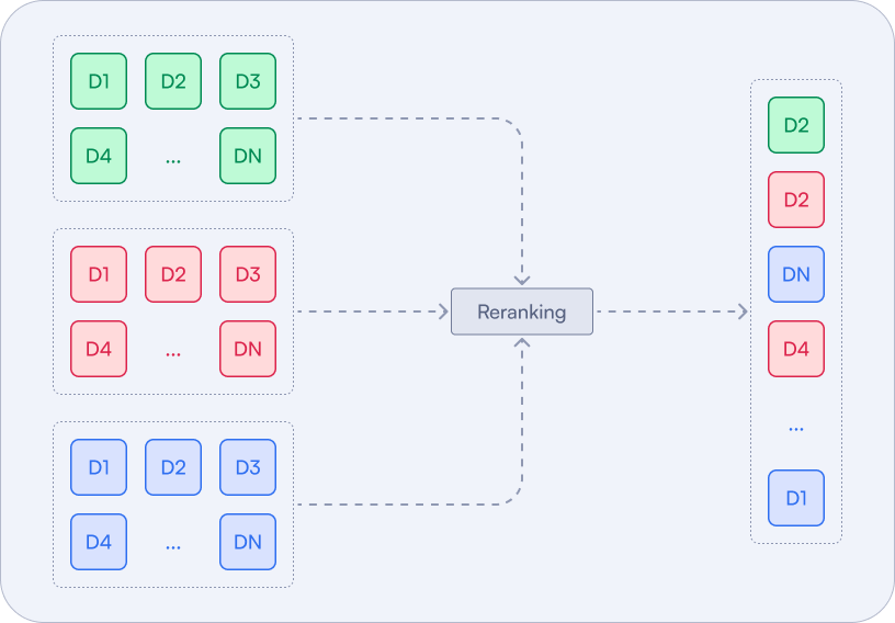
These methods are practically applicable only when used on a smaller subset of candidates returned by the faster search methods. Late interaction models, such as ColBERT, are way more efficient in this case, as they can be used to rerank the candidates without the need to access all the documents in the collection.
Example:
client.query_points(
       "collection-name",
       prefetch=prefetch, # Previous results
       query=late_vectors, # Colbert converted query
       using="colbertv2.0",
       with_payload=True,
       limit=10,
)
Learn more about Reranking.
Storage: Disk vs RAM

| Storage | Description |
|---|---|
| RAM | Crucial for fast access to frequently used data, such as indexed vectors. The amount of RAM required can be estimated based on your dataset size and dimensionality. For example, storing 1 million vectors with 1024 dimensions would require approximately 5.72 GB of RAM. |
| Disk | Suitable for less frequently accessed data, such as payloads and non-critical information. Disk-backed storage reduces memory demands but can introduce slight latency. |
Which Disk Type?
Local SSDs are recommended for optimal performance, as they provide the fastest query response times with minimal latency. While network-attached storage is also viable, it typically introduces additional latency that can affect performance, so local SSDs are preferred when possible, particularly for workloads requiring high-speed random access.
Memory Management for Vectors and Payload
As your data scales, effective resource management becomes crucial to keeping costs low while ensuring your application remains reliable and performant. One of the key areas to focus on is memory management.
Understanding how Qdrant handles memory can help you make informed decisions about scaling your vector database. Qdrant supports two main methods for storing vectors:
1. In-Memory Storage
- How it works: All data is stored in RAM, providing the fastest access times for queries and operations.
- When to use it: This setup is ideal for applications where performance is critical, and your RAM capacity can accommodate all data.
- Advantages: Maximum speed for queries and updates.
- Limitations: RAM usage can become a bottleneck as your dataset grows.
2. Memmap Storage
- How it works: Instead of loading all data into memory, memmap storage maps data files directly to a virtual address space on disk. The system’s page cache handles data access, making it highly efficient.
- When to use it: Perfect for storing large collections that exceed your available RAM while still maintaining near in-memory performance when enough RAM is available.
- Advantages: Balances performance and memory usage, allowing you to work with datasets larger than your physical RAM.
- Limitations: Slightly slower than pure in-memory storage but significantly more scalable.
To enable memmap vector storage in Qdrant, you can set the on_disk parameter to true when creating or updating a collection.
client.create_collection(
   collection_name="{collection_name}",
   vectors_config=models.VectorParams(
      …
      on_disk=True
   )
)
To do the same for payloads:
client.create_collection(
    collection_name="{collection_name}",
    on_disk_payload= True
)
The general guideline for selecting a storage method in Qdrant is to use InMemory storage when high performance is a priority, and sufficient RAM is available to accommodate the dataset. This approach ensures the fastest access speeds by keeping data readily accessible in memory.
However, for larger datasets or scenarios where memory is limited, Memmap and OnDisk storage are more suitable. These methods significantly reduce memory usage by storing data on disk while leveraging advanced techniques like page caching and indexing to maintain efficient and relatively fast data access.
Monitoring the Database

Continuous monitoring is essential for maintaining system health and identifying potential issues before they escalate. Tools like Prometheus and Grafana are widely used to achieve this.
- Prometheus: An open-source monitoring and alerting toolkit, Prometheus collects and stores metrics in a time-series database. It scrapes metrics from predefined endpoints and supports powerful querying and visualization capabilities.
- Grafana: Often paired with Prometheus, Grafana provides an intuitive interface for visualizing metrics and creating interactive dashboards.
Qdrant exposes metrics in the Prometheus/OpenMetrics format through the /metrics endpoint. Prometheus can scrape this endpoint to monitor various aspects of the Qdrant system.
For a local Qdrant instance, the metrics endpoint is typically available at:
http://localhost:6333/metrics
Here are some important metrics to monitor:
| Metric Name | Meaning | |
|---|---|---|
| collections_total | Total number of collections | |
| collections_vector_total | Total number of vectors in all collections | |
| rest_responses_avg_duration_seconds | Average response duration in REST API | |
| grpc_responses_avg_duration_seconds | Average response duration in gRPC API | |
| rest_responses_fail_total | Total number of failed responses (REST) |
Read more about Qdrant Open Source Monitoring and Qdrant Cloud Monitoring for managed clusters.
Recap: When Should You Optimize?

| Scenario | Description |
|---|---|
| When You Scale Up | As data grows and the request surge, optimizing resource usage ensures your systems stay responsive and cost-efficient, even under heavy loads. |
| If Facing Budget Constraints | Strike the perfect balance between performance and cost, cutting unnecessary expenses while maintaining essential capabilities. |
| You Need Better Performance | If you’re noticing slow query speeds, latency issues, or frequent timeouts, it’s time to fine-tune your resource allocation. |
| When System Stability is Paramount | To manage high-traffic environments you will need to prevent crashes or failures caused by resource exhaustion. |
Get the Cheatsheet
Want to download a printer-friendly version of this guide? Download it now..