Vector quantization is a data compression technique used to reduce the size of high-dimensional data. Compressing vectors reduces memory usage while maintaining nearly all of the essential information. This method allows for more efficient storage and faster search operations, particularly in large datasets.
When working with high-dimensional vectors, such as embeddings from providers like OpenAI, a single 1536-dimensional vector requires 6 KB of memory.

With 1 million vectors needing around 6 GB of memory, as your dataset grows to multiple millions of vectors, the memory and processing demands increase significantly.
To understand why this process is so computationally demanding, let’s take a look at the nature of the HNSW index.
The HNSW (Hierarchical Navigable Small World) index organizes vectors in a layered graph, connecting each vector to its nearest neighbors. At each layer, the algorithm narrows down the search area until it reaches the lower layers, where it efficiently finds the closest matches to the query.
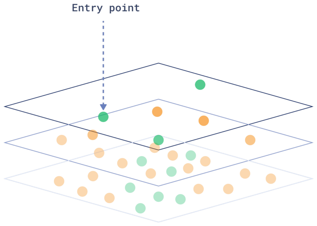
Each time a new vector is added, the system must determine its position in the existing graph, a process similar to searching. This makes both inserting and searching for vectors complex operations.
One of the key challenges with the HNSW index is that it requires a lot of random reads and sequential traversals through the graph. This makes the process computationally expensive, especially when you’re dealing with millions of high-dimensional vectors.
The system has to jump between various points in the graph in an unpredictable manner. This unpredictability makes optimization difficult, and as the dataset grows, the memory and processing requirements increase significantly.
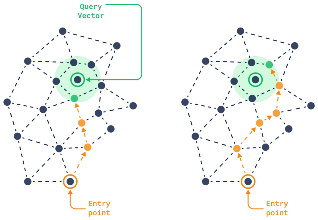
Since vectors need to be stored in fast storage like RAM or SSD for low-latency searches, as the size of the data grows, so does the cost of storing and processing it efficiently.
Quantization offers a solution by compressing vectors to smaller memory sizes, making the process more efficient.
There are several methods to achieve this, and here we will focus on three main ones:

1. What is Scalar Quantization?

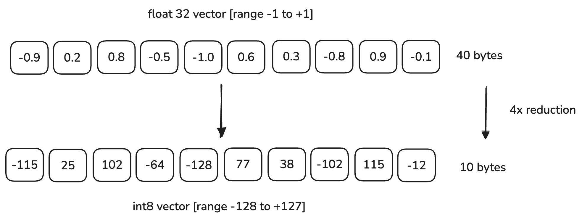
In Qdrant, each dimension is represented by a float32 value, which uses 4 bytes of memory. When using Scalar Quantization, we map our vectors to a range that the smaller int8 type can represent. An int8 is only 1 byte and can represent 256 values (from -128 to 127, or 0 to 255). This results in a 75% reduction in memory size.
For example, if our data lies in the range of -1.0 to 1.0, Scalar Quantization will transform these values to a range that int8 can represent, i.e., within -128 to 127. The system maps the float32 values into this range.
Here’s a simple linear example of what this process looks like:
To set up Scalar Quantization in Qdrant, you need to include the quantization_config section when creating or updating a collection:
PUT /collections/{collection_name}
{
    "vectors": {
      "size": 128,
      "distance": "Cosine"
    },
    "quantization_config": {
        "scalar": {
            "type": "int8",
            "quantile": 0.99,
            "always_ram": true
        }
    }
}
client.create_collection(
    collection_name="{collection_name}",
    vectors_config=models.VectorParams(size=128, distance=models.Distance.COSINE),
    quantization_config=models.ScalarQuantization(
        scalar=models.ScalarQuantizationConfig(
            type=models.ScalarType.INT8,
            quantile=0.99,
            always_ram=True,
        ),
    ),
)
The quantile parameter is used to calculate the quantization bounds. For example, if you specify a 0.99 quantile, the most extreme 1% of values will be excluded from the quantization bounds.
This parameter only affects the resulting precision, not the memory footprint. You can adjust it if you experience a significant decrease in search quality.
Scalar Quantization is a great choice if you’re looking to boost search speed and compression without losing much accuracy. It also slightly improves performance, as distance calculations (such as dot product or cosine similarity) using int8 values are computationally simpler than using float32 values.
While the performance gains of Scalar Quantization may not match those achieved with Binary Quantization (which we’ll discuss later), it remains an excellent default choice when Binary Quantization isn’t suitable for your use case.
2. What is Binary Quantization?

Binary Quantization is an excellent option if you’re looking to reduce memory usage while also achieving a significant boost in speed. It works by converting high-dimensional vectors into simple binary (0 or 1) representations.
- Values greater than zero are converted to 1.
- Values less than or equal to zero are converted to 0.
Let’s consider our initial example of a 1536-dimensional vector that requires 6 KB of memory (4 bytes for each float32 value).
After Binary Quantization, each dimension is reduced to 1 bit (1/8 byte), so the memory required is:
This leads to a 32x memory reduction.

Qdrant automates the Binary Quantization process during indexing. As vectors are added to your collection, each 32-bit floating-point component is converted into a binary value according to the configuration you define.
Here’s how you can set it up:
PUT /collections/{collection_name}
{
    "vectors": {
      "size": 1536,
      "distance": "Cosine"
    },
    "quantization_config": {
        "binary": {
            "always_ram": true
        }
    }
}
client.create_collection(
    collection_name="{collection_name}",
    vectors_config=models.VectorParams(size=1536, distance=models.Distance.COSINE),
    quantization_config=models.BinaryQuantization(
        binary=models.BinaryQuantizationConfig(
            always_ram=True,
        ),
    ),
)
Binary Quantization is by far the quantization method that provides the most significant processing speed gains compared to Scalar and Product Quantizations. This is because the binary representation allows the system to use highly optimized CPU instructions, such as XOR and Popcount, for fast distance computations.
It can speed up search operations by up to 40x, depending on the dataset and hardware.
Not all models are equally compatible with Binary Quantization, and in the comparison above, we are only using models that are compatible. Some models may experience a greater loss in accuracy when quantized. We recommend using Binary Quantization with models that have at least 1024 dimensions to minimize accuracy loss.
The models that have shown the best compatibility with this method include:
- OpenAI text-embedding-ada-002 (1536 dimensions)
- Cohere AI embed-english-v2.0 (4096 dimensions)
These models demonstrate minimal accuracy loss while still benefiting from substantial speed and memory gains.
Even though Binary Quantization is incredibly fast and memory-efficient, the trade-offs are in precision and model compatibility, so you may need to ensure search quality using techniques like oversampling and rescoring.
If you’re interested in exploring Binary Quantization in more detail—including implementation examples, benchmark results, and usage recommendations—check out our dedicated article on Binary Quantization - Vector Search, 40x Faster.
3. What is Product Quantization?

Product Quantization is a method used to compress high-dimensional vectors by representing them with a smaller set of representative points.
The process begins by splitting the original high-dimensional vectors into smaller sub-vectors. Each sub-vector represents a segment of the original vector, capturing different characteristics of the data.

For each sub-vector, a separate codebook is created, representing regions in the data space where common patterns occur.
The codebook in Qdrant is trained automatically during the indexing process. As vectors are added to the collection, Qdrant uses your specified quantization settings in the quantization_config to build the codebook and quantize the vectors. Here’s how you can set it up:
PUT /collections/{collection_name}
{
    "vectors": {
      "size": 1024,
      "distance": "Cosine"
    },
    "quantization_config": {
        "product": {
            "compression": "x32",
            "always_ram": true
        }
    }
}
client.create_collection(
    collection_name="{collection_name}",
    vectors_config=models.VectorParams(size=1024, distance=models.Distance.COSINE),
    quantization_config=models.ProductQuantization(
        product=models.ProductQuantizationConfig(
            compression=models.CompressionRatio.X32,
            always_ram=True,
        ),
    ),
)
Each region in the codebook is defined by a centroid, which serves as a representative point summarizing the characteristics of that region. Instead of treating every single data point as equally important, we can group similar sub-vectors together and represent them with a single centroid that captures the general characteristics of that group.
The centroids used in Product Quantization are determined using the K-means clustering algorithm.
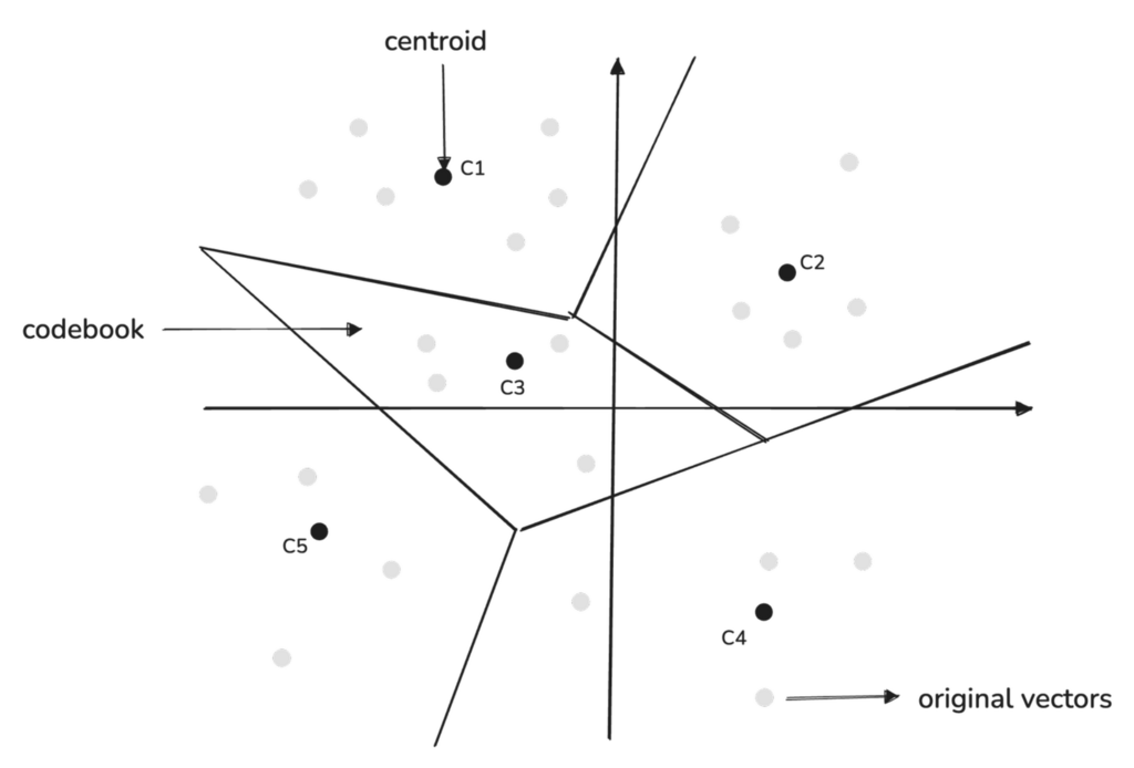
Qdrant always selects K = 256 as the number of centroids in its implementation, based on the fact that 256 is the maximum number of unique values that can be represented by a single byte.
This makes the compression process efficient because each centroid index can be stored in a single byte.
The original high-dimensional vectors are quantized by mapping each sub-vector to the nearest centroid in its respective codebook.
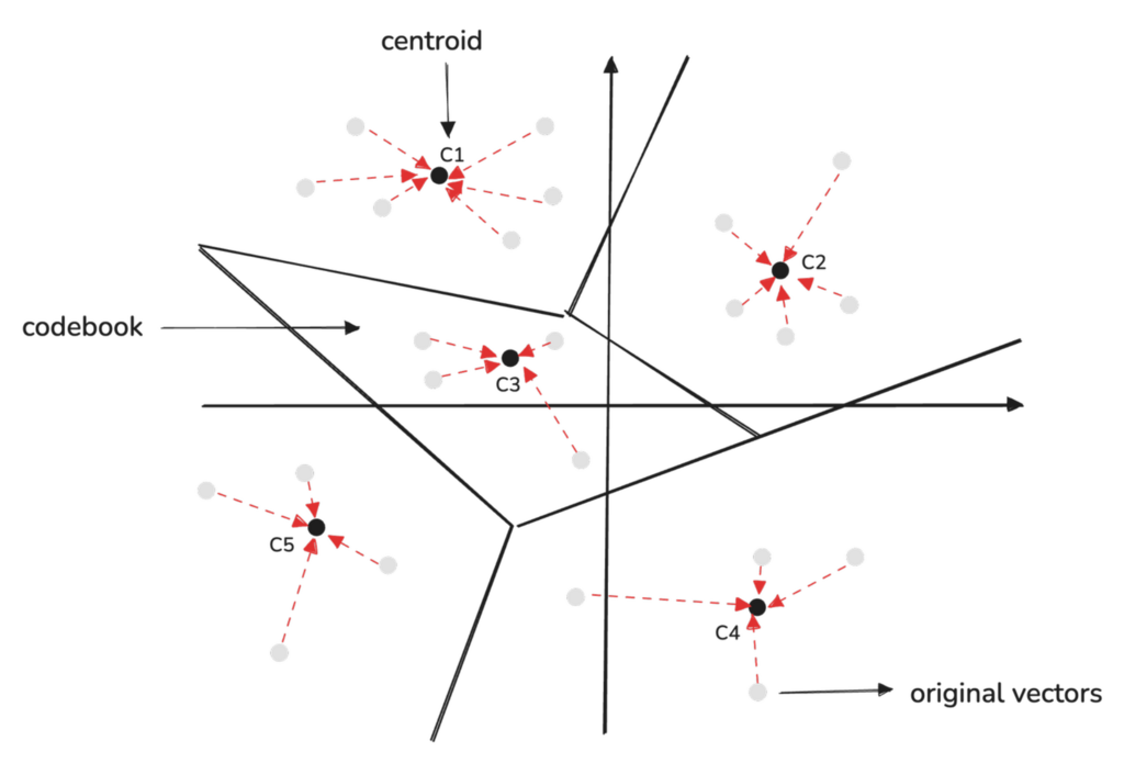
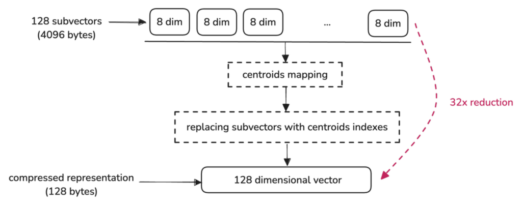
The compressed vector stores the index of the closest centroid for each sub-vector.
Here’s how a 1024-dimensional vector, originally taking up 4096 bytes, is reduced to just 128 bytes by representing it as 128 indexes, each pointing to the centroid of a sub-vector:
After setting up quantization and adding your vectors, you can perform searches as usual. Qdrant will automatically use the quantized vectors, optimizing both speed and memory usage. Optionally, you can enable rescoring for better accuracy.
POST /collections/{collection_name}/points/search
{
    "query": [0.22, -0.01, -0.98, 0.37],
    "params": {
        "quantization": {
            "rescore": true
        }
    },
    "limit": 10
}
client.query_points(
    collection_name="my_collection",
    query_vector=[0.22, -0.01, -0.98, 0.37],  # Your query vector
    search_params=models.SearchParams(
        quantization=models.QuantizationSearchParams(
            rescore=True  # Enables rescoring with original vectors
        )
    ),
    limit=10  # Return the top 10 results
)
Product Quantization can significantly reduce memory usage, potentially offering up to 64x compression in certain configurations. However, it’s important to note that this level of compression can lead to a noticeable drop in quality.
If your application requires high precision or real-time performance, Product Quantization may not be the best choice. However, if memory savings are critical and some accuracy loss is acceptable, it could still be an ideal solution.
Here’s a comparison of speed, accuracy, and compression for all three methods, adapted from Qdrant’s documentation:
| Quantization method | Accuracy | Speed | Compression |
|---|---|---|---|
| Scalar | 0.99 | up to x2 | 4 |
| Product | 0.7 | 0.5 | up to 64 |
| Binary | 0.95* | up to x40 | 32 |
* - for compatible models
For a more in-depth understanding of the benchmarks you can expect, check out our dedicated article on Product Quantization in Vector Search.
Rescoring, Oversampling, and Reranking
When we use quantization methods like Scalar, Binary, or Product Quantization, we’re compressing our vectors to save memory and improve performance. However, this compression removes some detail from the original vectors.
This can slightly reduce the accuracy of our similarity searches because the quantized vectors are approximations of the original data. To mitigate this loss of accuracy, you can use oversampling and rescoring, which help improve the accuracy of the final search results.
The original vectors are never deleted during this process, and you can easily switch between quantization methods or parameters by updating the collection configuration at any time.
Here’s how the process works, step by step:
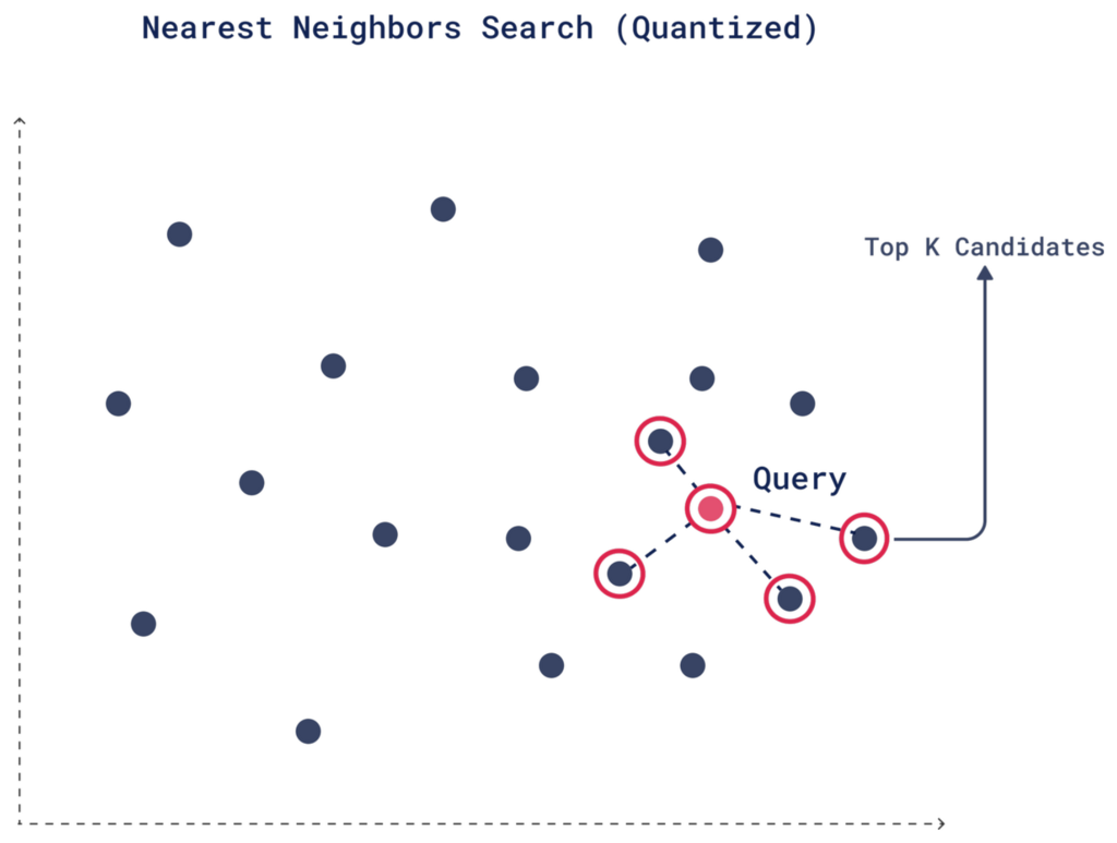
1. Initial Quantized Search
When you perform a search, Qdrant retrieves the top candidates using the quantized vectors based on their similarity to the query vector, as determined by the quantized data. This step is fast because we’re using the quantized vectors.
2. Oversampling
Oversampling is a technique that helps compensate for any precision lost due to quantization. Since quantization simplifies vectors, some relevant matches could be missed in the initial search. To avoid this, you can retrieve more candidates, increasing the chances that the most relevant vectors make it into the final results.
You can control the number of extra candidates by setting an oversampling parameter. For example, if your desired number of results (limit) is 4 and you set an oversampling factor of 2, Qdrant will retrieve 8 candidates (4 × 2).
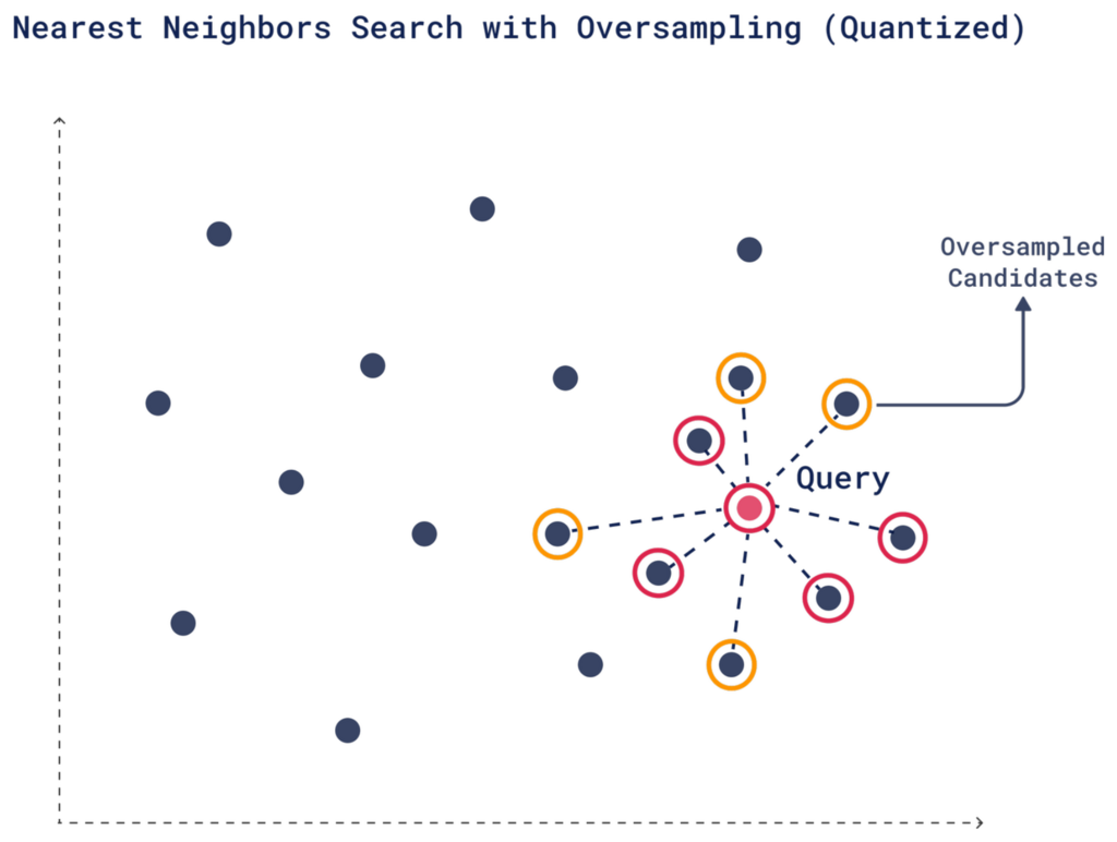
You can adjust the oversampling factor to control how many extra vectors Qdrant includes in the initial pool. More candidates mean a better chance of obtaining high-quality top-K results, especially after rescoring with the original vectors.
3. Rescoring with Original Vectors
After oversampling to gather more potential matches, each candidate is re-evaluated based on additional criteria to ensure higher accuracy and relevance to the query.
The rescoring process maps the quantized vectors to their corresponding original vectors, allowing you to consider factors like context, metadata, or additional relevance that wasn’t included in the initial search, leading to more accurate results.
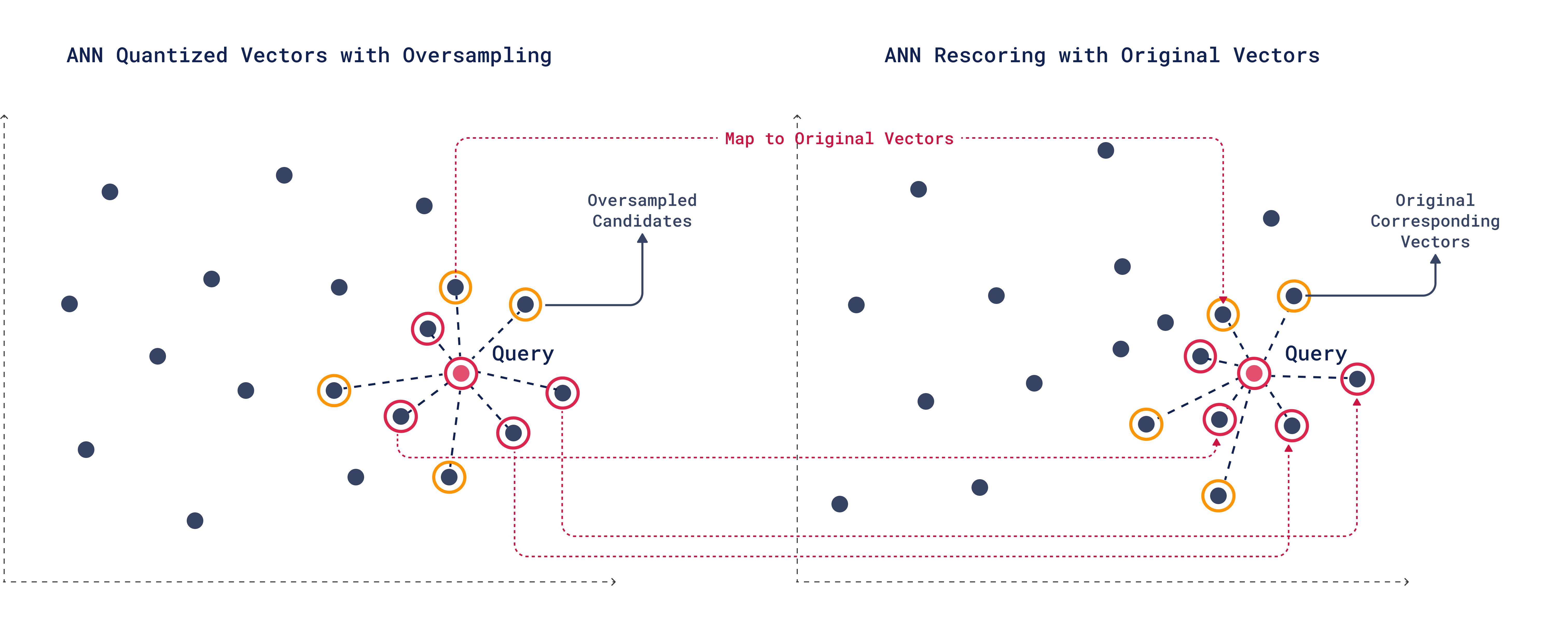
During rescoring, one of the lower-ranked candidates from oversampling might turn out to be a better match than some of the original top-K candidates.
Even though rescoring uses the original, larger vectors, the process remains much faster because only a very small number of vectors are read. The initial quantized search already identifies the specific vectors to read, rescore, and rerank.
4. Reranking
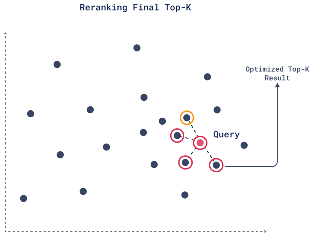
With the new similarity scores from rescoring, reranking is where the final top-K candidates are determined based on the updated similarity scores.
For example, in our case with a limit of 4, a candidate that ranked 6th in the initial quantized search might improve its score after rescoring because the original vectors capture more context or metadata. As a result, this candidate could move into the final top 4 after reranking, replacing a less relevant option from the initial search.
Here’s how you can set it up:
POST /collections/{collection_name}/points/search


{
  "query": [0.22, -0.01, -0.98, 0.37],
  "params": {
    "quantization": {
      "rescore": true,
      "oversampling": 2
    }
  },
  "limit": 4
}
client.query_points(
    collection_name="my_collection",
    query_vector=[0.22, -0.01, -0.98, 0.37],
    search_params=models.SearchParams(
        quantization=models.QuantizationSearchParams(
            rescore=True,   # Enables rescoring with original vectors
            oversampling=2  # Retrieves extra candidates for rescoring
        )
    ),
    limit=4  # Desired number of final results
)
You can adjust the oversampling factor to find the right balance between search speed and result accuracy.
If quantization is impacting performance in an application that requires high accuracy, combining oversampling with rescoring is a great choice. However, if you need faster searches and can tolerate some loss in accuracy, you might choose to use oversampling without rescoring, or adjust the oversampling factor to a lower value.
Distributing Resources Between Disk & Memory
Qdrant stores both the quantized and original vectors. When you enable quantization, both the original and quantized vectors are stored in RAM by default. You can move the original vectors to disk to significantly reduce RAM usage and lower system costs. Simply enabling quantization is not enough—you need to explicitly move the original vectors to disk by setting on_disk=True.
Here’s an example configuration:
PUT /collections/{collection_name}
{
  "vectors": {
    "size": 1536,
    "distance": "Cosine",
    "on_disk": true  # Move original vectors to disk
  },
  "quantization_config": {
    "binary": {
      "always_ram": true  # Store only quantized vectors in RAM
    }
  }
}
client.update_collection(
    collection_name="my_collection",
    vectors_config=models.VectorParams(
        size=1536,
        distance=models.Distance.COSINE,
        on_disk=True  # Move original vectors to disk
    ),
    quantization_config=models.BinaryQuantization(
        binary=models.BinaryQuantizationConfig(
            always_ram=True  # Store only quantized vectors in RAM
        )
    )
)
Without explicitly setting on_disk=True, you won’t see any RAM savings, even with quantization enabled. So, make sure to configure both storage and quantization options based on your memory and performance needs. If your storage has high disk latency, consider disabling rescoring to maintain speed.
Speeding Up Rescoring with io_uring
When dealing with large collections of quantized vectors, frequent disk reads are required to retrieve both original and compressed data for rescoring operations. While mmap helps with efficient I/O by reducing user-to-kernel transitions, rescoring can still be slowed down when working with large datasets on disk due to the need for frequent disk reads.
On Linux-based systems, io_uring allows multiple disk operations to be processed in parallel, significantly reducing I/O overhead. This optimization is particularly effective during rescoring, where multiple vectors need to be re-evaluated after the initial search. With io_uring, Qdrant can retrieve and rescore vectors from disk in the most efficient way, improving overall search performance.
When you perform vector quantization and store data on disk, Qdrant often needs to access multiple vectors in parallel. Without io_uring, this process can be slowed down due to the system’s limitations in handling many disk accesses.
To enable io_uring in Qdrant, add the following to your storage configuration:
storage:
  async_scorer: true  # Enable io_uring for async storage
Without this configuration, Qdrant will default to using mmap for disk I/O operations.
For more information and benchmarks comparing io_uring with traditional I/O approaches like mmap, check out Qdrant’s io_uring implementation article.
Performance of Quantized vs. Non-Quantized Data
Qdrant uses the quantized vectors by default if they are available. If you want to evaluate how quantization affects your search results, you can temporarily disable it to compare results from quantized and non-quantized searches. To do this, set ignore: true in the query:
POST /collections/{collection_name}/points/query
{
    "query": [0.22, -0.01, -0.98, 0.37],
    "params": {
        "quantization": {
            "ignore": true,
        }
    },
    "limit": 4
}
client.query_points(
    collection_name="{collection_name}",
    query=[0.22, -0.01, -0.98, 0.37],
    search_params=models.SearchParams(
        quantization=models.QuantizationSearchParams(
            ignore=True
        )
    ),
)
Switching Between Quantization Methods
Not sure if you’ve chosen the right quantization method? In Qdrant, you have the flexibility to remove quantization and rely solely on the original vectors, adjust the quantization type, or change compression parameters at any time without affecting your original vectors.
To switch to binary quantization and adjust the compression rate, for example, you can update the collection’s quantization configuration using the update_collection method:
PUT /collections/{collection_name}
{
  "vectors": {
    "size": 1536,
    "distance": "Cosine"
  },
  "quantization_config": {
    "binary": {
      "always_ram": true,
      "compression_rate": 0.8  # Set the new compression rate
    }
  }
}
client.update_collection(
    collection_name="my_collection",
    quantization_config=models.BinaryQuantization(
        binary=models.BinaryQuantizationConfig(
            always_ram=True,  # Store only quantized vectors in RAM
            compression_rate=0.8  # Set the new compression rate
        )
    ),
)
If you decide to turn off quantization and use only the original vectors, you can remove the quantization settings entirely with quantization_config=None:
PUT /collections/my_collection
{
  "vectors": {
    "size": 1536,
    "distance": "Cosine"
  },
  "quantization_config": null  # Remove quantization and use original vectors only
}
client.update_collection(
    collection_name="my_collection",
    quantization_config=None  # Remove quantization and rely on original vectors only
)
Wrapping Up

Quantization methods like Scalar, Product, and Binary Quantization offer powerful ways to optimize memory usage and improve search performance when dealing with large datasets of high-dimensional vectors. Each method comes with its own trade-offs between memory savings, computational speed, and accuracy.
Here are some final thoughts to help you choose the right quantization method for your needs:
| Quantization Method | Key Features | When to Use |
|---|---|---|
| Binary Quantization | • Fastest method and most memory-efficient • Up to 40x faster search and 32x reduced memory footprint | • Use with tested models like OpenAI’s text-embedding-ada-002 and Cohere’s embed-english-v2.0• When speed and memory efficiency are critical |
| Scalar Quantization | • Minimal loss of accuracy • Up to 4x reduced memory footprint | • Safe default choice for most applications. • Offers a good balance between accuracy, speed, and compression. |
| Product Quantization | • Highest compression ratio • Up to 64x reduced memory footprint | • When minimizing memory usage is the top priority • Acceptable if some loss of accuracy and slower indexing is tolerable |
Learn More
If you want to learn more about improving accuracy, memory efficiency, and speed when using quantization in Qdrant, we have a dedicated Quantization tips section in our docs that explains all the quantization tips you can use to enhance your results.
Learn more about optimizing real-time precision with oversampling in Binary Quantization by watching this interview with Qdrant’s CTO, Andrey Vasnetsov:
Stay up-to-date on the latest in vector search and quantization, share your projects, ask questions, join our vector search community!


