Large-Scale Search in Qdrant
| Time: 2 days | Level: Advanced |
|---|
In this tutorial, we will describe an approach to upload, index, and search a large volume of data cost-efficiently, on an example of the real-world dataset LAION-400M.
The goal of this tutorial is to demonstrate what minimal amount of resources is required to index and search a large dataset, while still maintaining a reasonable search latency and accuracy.
All relevant code snippets are available in the GitHub repository.
The recommended Qdrant version for this tutorial is v1.13.5 and higher.
Dataset
The dataset we will use is LAION-400M, a collection of approximately 400 million vectors obtained from images extracted from a Common Crawl dataset. Each vector is 512-dimensional and generated using a CLIP model.
Vectors are associated with a number of metadata fields, such as url, caption, LICENSE, etc.
The overall payload size is approximately 200 GB, and the vectors are 400 GB.
The dataset is available in the form of 409 chunks, each containing approximately 1M vectors. We will use the following python script to upload dataset chunks one by one.
Hardware
After some initial experiments, we figured out a minimal hardware configuration for the task:
- 8 CPU cores
- 64Gb RAM
- 650Gb Disk space
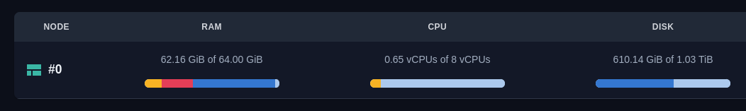
Hardware configuration
This configuration is enough to index and explore the dataset in a single-user mode; latency is reasonable enough to build interactive graphs and navigate in the dashboard.
Naturally, you might need more CPU cores and RAM for production-grade configurations.
It is important to ensure high network bandwidth for this experiment so you are running the client and server in the same region.
Uploading and Indexing
We will use the following python script to upload dataset chunks one by one.
export QDRANT_URL="https://xxxx-xxxx.xxxx.cloud.qdrant.io"
export QDRANT_API_KEY="xxxx-xxxx-xxxx-xxxx"

python upload.py
This script will download chunks of the LAION dataset one by one and upload them to Qdrant. Intermediate data is not persisted on disk, so the script doesn’t require much disk space on the client side.
Let’s take a look at the collection configuration we used:
client.create_collection(
        QDRANT_COLLECTION_NAME,
        vectors_config=models.VectorParams(
            size=512, # CLIP model output size
            distance=models.Distance.COSINE, # CLIP model uses cosine distance
            datatype=models.Datatype.FLOAT16, # We only need 16 bits for float, otherwise disk usage would be 800Gb instead of 400Gb
            on_disk=True # We don't need original vectors in RAM
        ),
        # Even though CLIP vectors don't work well with binary quantization, out of the box,
        # we can rely on query-time oversampling to get more accurate results
        quantization_config=models.BinaryQuantization(
            binary=models.BinaryQuantizationConfig(
                always_ram=True,
            )
        ),
        optimizers_config=models.OptimizersConfigDiff(
            # Bigger size of segments are desired for faster search
            # However it might be slower for indexing
            max_segment_size=5_000_000,
        ),
        # Having larger M value is desirable for higher accuracy,
        # but in our case we care more about memory usage
        # We could still achieve reasonable accuracy even with M=6 + oversampling
        hnsw_config=models.HnswConfigDiff(
            m=6, # decrease M for lower memory usage
            on_disk=False
        ),
    )
There are a few important points to note:
- We use
FLOAT16datatype for vectors, which allows us to store vectors in half the size compared toFLOAT32. There are no significant accuracy losses for this dataset. - We use
BinaryQuantizationwithalways_ram=Trueto enable query-time oversampling. This allows us to get an accurate and resource-efficient search, even though 512d CLIP vectors don’t work well with binary quantization out of the box. - We use
HnswConfigwithm=6to reduce memory usage. We will look deeper into memory usage in the next section.
Goal of this configuration is to ensure that prefetch component of the search never needs to load data from disk, and at least a minimal version of vectors and vector index is always in RAM. The second stage of the search can explicitly determine how many times we can afford to load data from a disk.
In our experiment, the upload process was going at 5000 points per second. The indexation process was going in parallel with the upload and was happening at the rate of approximately 4000 points per second.
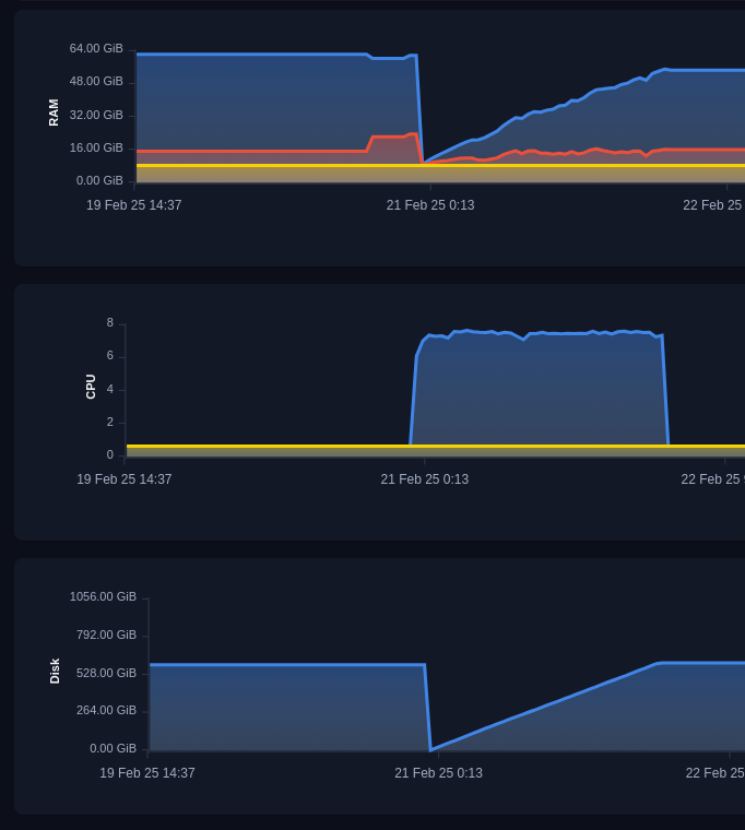
Upload and indexation process
Memory Usage
After the upload and indexation process is finished, let’s take a detailed look at the memory usage of the Qdrant server.
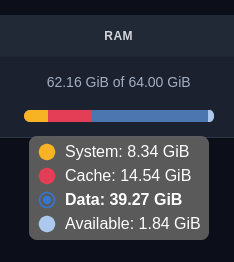
Memory usage
On the high level, memory usage consists of 3 components:
- System memory - 8.34Gb - this is memory reserved for internal systems and OS, it doesn’t depend on the dataset size.
- Data memory - 39.27Gb - this is a resident memory of qdrant process, it can’t be evicter and qdrant process will crash if it exceeds the limit.
- Cache memory - 14.54Gb - this is a disk cache qdrant uses. It is necessary for fast search but can be evicted if needed.
The most interest for us is Data and Cache memory. Let’s look what exactly is stored in these components.
In our scenario, Qdrant uses memory to store the following components:
- Storing vectors
- Storing vector index
- Storing information about IDs and versions of points
Size of vectors
In our scenario, we store only quantized vectors in RAM, so it is relatively easy to calculate the required size:
400_000_000 * 512d / 8 bits / 1024 (Kb) / 1024 (Mb) / 1024 (Gb) = 23.84Gb
Size of vector index
Vector index is a bit more complicated, as it is not a simple matrix.
Internally, it is stored as a list of connections in a graph, and each connection is a 4-byte integer.
The number of connections is defined by the M parameter of the HNSW index, and in our case, it is 6 on the high level and 2 x M on level 0.
This gives us the following estimation:
400_000_000 * (6 * 2) * 4 bytes / 1024 (Kb) / 1024 (Mb) / 1024 (Gb) = 17.881Gb
In practice the size of index is a bit smaller due to the compression we implemented in Qdrant v1.13.0, but it is still a good estimation.
The HNSW index in Qdrant is stored as a mmap, and it can be evicted from RAM if needed.
So, the memory consumption of HNSW falls under the category of Cache memory.
Size of IDs and versions
Qdrant must store additional information about each point, such as ID and version. This information is needed on each request, so it is very important to keep it in RAM for fast access.
Let’s take a look at Qdrant internals to understand how much memory is required for this information.
// This is s simplified version of the IdTracker struct
// It omits all optimizations and small details,
// but gives a good estimation of memory usage
IdTracker {
    // Mapping of internal id to version (u64), compressed to 4 bytes
    // Required for versioning and conflict resolution between segments
    internal_to_version, // 400M x 4 = 1.5Gb

    // Mapping of external id to internal id, 4 bytes per point.
    // Required to determine original point ID after search inside the segment
    internal_to_external: Vec<u128>, // 400M x 16 = 6.4Gb

    // Mapping of external id to internal id. For numeric ids it uses 8 bytes,
    //  UUIDs are stored as 16 bytes.
    // Required to determine sequential point ID inside the segment
    external_to_internal: Vec<u64, u32>, // 400M x (8 + 4) = 4.5Gb
}
In the v1.13.5 we introduced a significant optimization to reduce the memory usage of IdTracker by approximately 2 times.
So the total memory usage of IdTracker in our case is approximately 12.4Gb.
So total expected RAM usage of Qdrant server in our case is approximately 23.84Gb + 17.881Gb + 12.4Gb = 54.121Gb, which is very close to the actual memory usage we observed: 39.27Gb + 14.54Gb = 53.81Gb.
We had to apply some simplifications to the estimations, but they are good enough to understand the memory usage of the Qdrant server.
Search
After the dataset is uploaded and indexed, we can start searching for similar vectors.
We can start by exploring the dataset in Web-UI. So you can get an intuition into the search performance, not just table numbers.

Web-UI Bear image
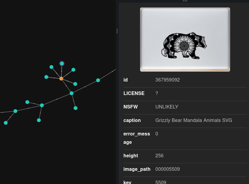
Web-UI similar Bear image
Web-UI default requests do not use oversampling, but the observable results are still good enough to see the resemblance between images.
Ground truth data
However, to estimate the search performance more accurately, we need to compare search results with the ground truth. Unfortunately, the LAION dataset doesn’t contain usable ground truth, so we had to generate it ourselves.
To do this, we need to perform a full-scan search for each vector in the dataset and store the results in a separate file. Unfortunately, this process is very time-consuming and requires a lot of resources, so we had to limit the number of queries to 100, we provide a ready-to-use ground truth file and the script to generate it (requires 512Gb RAM machine and about 20 hours of execution time).
Our ground truth file contains 100 queries, each with 50 results. The first 100 vectors of the dataset itself were used to generate queries.
Search Query
To precisely control the amount of oversampling, we will use the following search query:
limit = 50
rescore_limit = 1000 # oversampling factor is 20

query = vectors[query_id] # One of existing vectors

response = client.query_points(
        collection_name=QDRANT_COLLECTION_NAME,
        query=query,
        limit=limit,
        # Go to disk
        search_params=models.SearchParams(
            quantization=models.QuantizationSearchParams(
                rescore=True,
            ),
        ),
        # Prefetch is performed using only in-RAM data,
        # so querying even large amount of data is fast
        prefetch=models.Prefetch(
            query=query,
            limit=rescore_limit,
            params=models.SearchParams(
                quantization=models.QuantizationSearchParams(
                    # Avoid rescoring in prefetch
                    # We should do it explicitly on the second stage
                    rescore=False,
                ),
            )
        )
    )
As you can see, this query contains two stages:
- First stage is a prefetch, which is performed using only in-RAM data. It is very fast and allows us to get a large amount of candidates.
- The second stage is a rescore, which is performed with full-size vectors stored on disks.
By using 2-stage search we can precisely control the amount of data loaded from disk and ensure the balance between search speed and accuracy.
You can find the complete code of the search process in the eval.py
Performance tweak
One important performance tweak we found useful for this dataset is to enable Async IO in Qdrant.
By default, Qdrant uses synchronous IO, which is good for in-memory datasets but can be a bottleneck when we want to read a lot of data from a disk.
Async IO (implemented with io_uring) allows to send parallel requests to the disk and saturate the disk bandwidth.
This is exactly what we are looking for when performing large-scale re-scoring with original vectors.
Instead of reading vectors one by one and waiting for the disk response 1000 times, we can send 1000 requests to the disk and wait for all of them to complete. This allows us to saturate the disk bandwidth and get faster results.
To enable Async IO in Qdrant, you need to set the following environment variable:
QDRANT__STORAGE__PERFORMANCE__ASYNC_SCORER=true
Or set parameter in config file:
storage:
  performance:
    async_scorer: true
In Qdrant Managed cloud Async IO can be enabled via Advanced optimizations section in cluster Configuration tab.
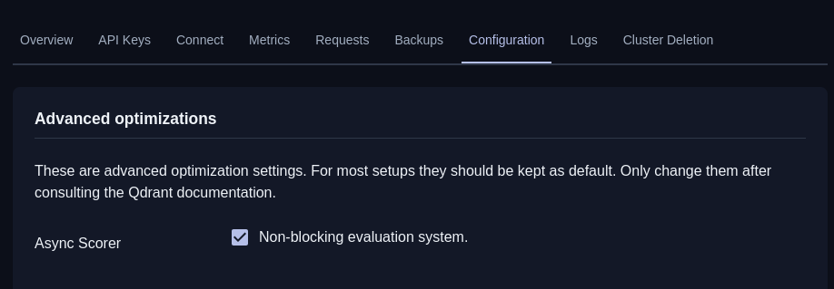
Async IO configuration in Cloud
Running search requests
Once all the preparations are done, we can run the search requests and evaluate the results.
You can find the full code of the search process in the eval.py
This script will run 100 search requests with configured oversampling factor and compare the results with the ground truth.
python eval.py --rescore_limit 1000
In our request we achieved the following results:
| Rescore Limit | Precision@50 | Time per request |
|---|---|---|
| 1000 | 75.2% | 0.7s |
| 5000 | 81.0% | 2.2s |
Additional experiments with m=16 demonstrated that we can achieve 85% precision with rescore_limit=1000, but they would require slightly more memory.
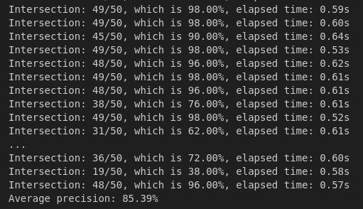
Log of search evaluation
Conclusion
In this tutorial we demonstrated how to upload, index and search a large dataset in Qdrant cost-efficiently. Binary quantization can be applied even on 512d vectors, if combined with query-time oversampling.
Qdrant allows to precisely control where each part of storage is located, which allows to achieve a good balance between search speed and memory usage.
Potential improvements
In this experiment, we investigated in detail which parts of the storage are responsible for memory usage and how to control them.
One especially interesting part is the VectorIndex component, which is responsible for storing the graph of connections between vectors.
In our further research, we will investigate the possibility of making HNSW more disk-friendly so it can be offloaded to disk without significant performance losses.