An Introduction to Vector Databases

Most of the millions of terabytes of data we generate each day is unstructured. Think of the meal photos you snap, the PDFs shared at work, or the podcasts you save but may never listen to. None of it fits neatly into rows and columns.
Unstructured data lacks a strict format or schema, making it challenging for conventional databases to manage. Yet, this unstructured data holds immense potential for AI, machine learning, and modern search engines.
A Vector Database is a specialized system designed to efficiently handle high-dimensional vector data. It excels at indexing, querying, and retrieving this data, enabling advanced analysis and similarity searches that traditional databases cannot easily perform.
The Challenge with Traditional Databases
Traditional OLTP and OLAP databases have been the backbone of data storage for decades. They are great at managing structured data with well-defined schemas, like name, address, phone number, and purchase history.
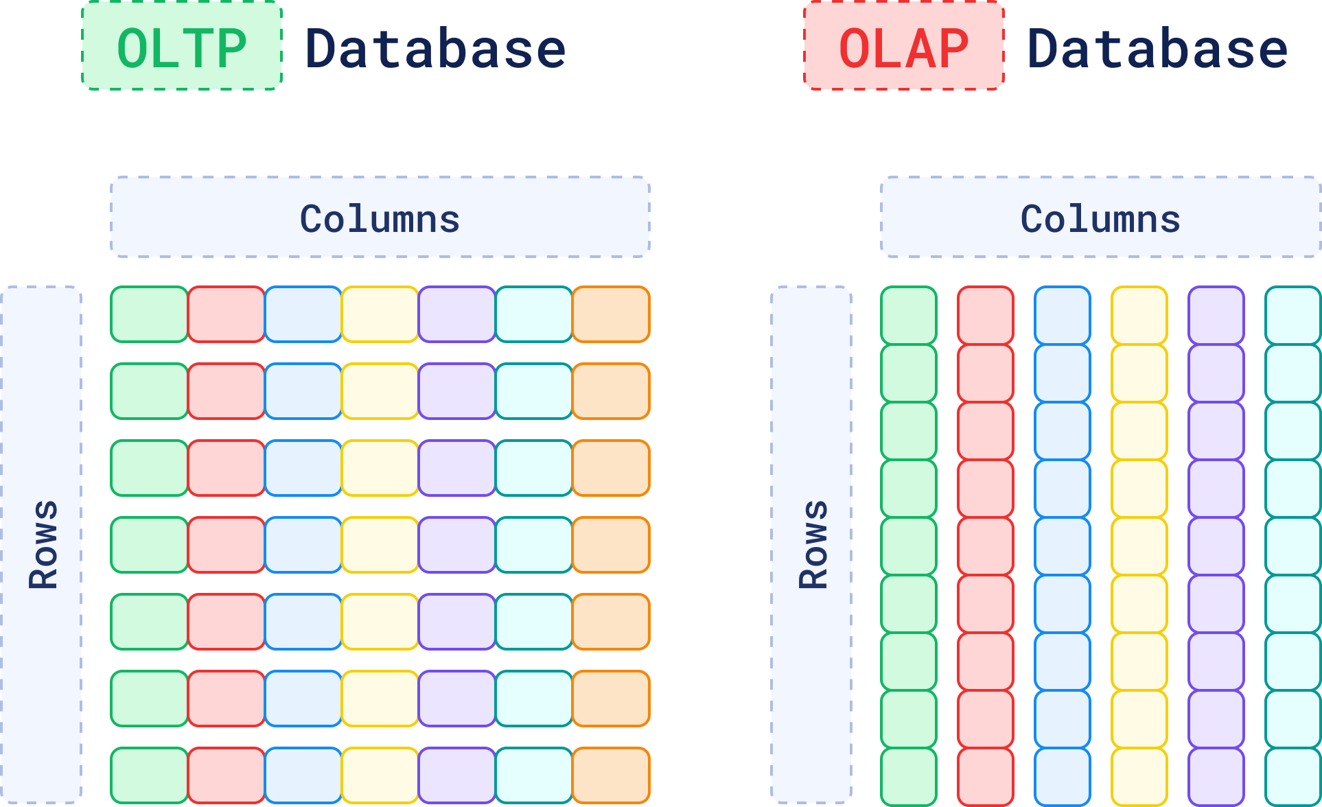
But when data can’t be easily categorized, like the content inside a PDF file, things start to get complicated.
You can always store the PDF file as raw data, perhaps with some metadata attached. However, the database still wouldn’t be able to understand what’s inside the document, categorize it, or even search for the information that it contains.
Also, this applies to more than just PDF documents. Think about the vast amounts of text, audio, and image data you generate every day. If a database can’t grasp the meaning of this data, how can you search for or find relationships within the data?
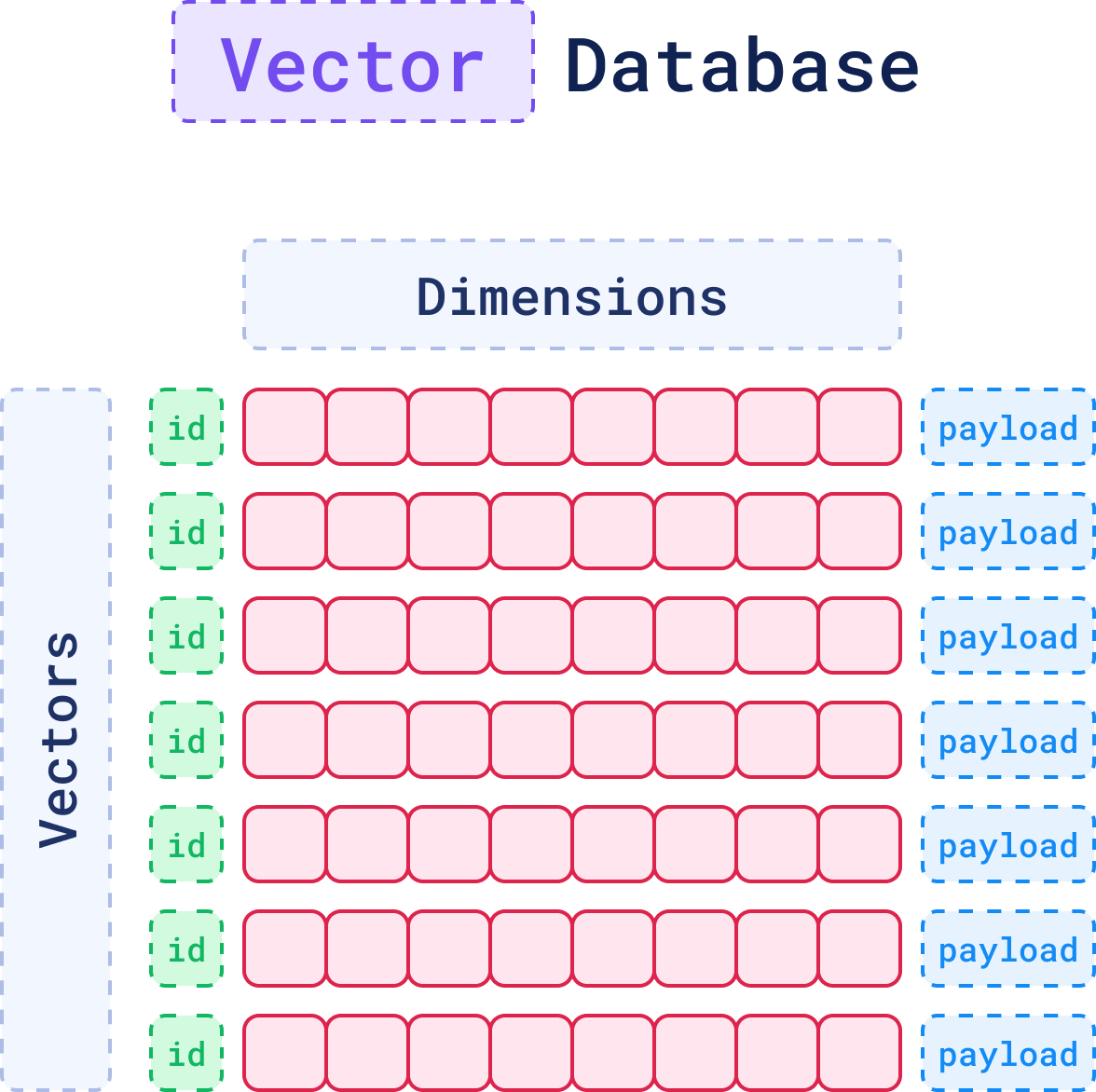
Vector databases allow you to understand the context or conceptual similarity of unstructured data by representing them as vectors, enabling advanced analysis and retrieval based on data similarity.
When to Use a Vector Database
Not sure if you should use a vector database or a traditional database? This chart may help.
| Feature | OLTP Database | OLAP Database | Vector Database |
|---|---|---|---|
| Data Structure | Rows and columns | Rows and columns | Vectors |
| Type of Data | Structured | Structured/Partially Unstructured | Unstructured |
| Query Method | SQL-based (Transactional Queries) | SQL-based (Aggregations, Analytical Queries) | Vector Search (Similarity-Based) |
| Storage Focus | Schema-based, optimized for updates | Schema-based, optimized for reads | Context and Semantics |
| Performance | Optimized for high-volume transactions | Optimized for complex analytical queries | Optimized for unstructured data retrieval |
| Use Cases | Inventory, order processing, CRM | Business intelligence, data warehousing | Similarity search, recommendations, RAG, anomaly detection, etc. |
What Is a Vector?

When a machine needs to process unstructured data - an image, a piece of text, or an audio file, it first has to translate that data into a format it can work with: vectors.
A vector is a numerical representation of data that can capture the context and semantics of data.
When you deal with unstructured data, traditional databases struggle to understand its meaning. However, a vector can translate that data into something a machine can process. For example, a vector generated from text can represent relationships and meaning between words, making it possible for a machine to compare and understand their context.
There are three key elements that define a vector in a vector database: the ID, the dimensions, and the payload. These components work together to represent a vector effectively within the system. Together, they form a point, which is the core unit of data stored and retrieved in a vector database.

Each one of these parts plays an important role in how vectors are stored, retrieved, and interpreted. Let’s see how.
1. The ID: Your Vector’s Unique Identifier
Just like in a relational database, each vector in a vector database gets a unique ID. Think of it as your vector’s name tag, a primary key that ensures the vector can be easily found later. When a vector is added to the database, the ID is created automatically.
While the ID itself doesn’t play a part in the similarity search (which operates on the vector’s numerical data), it is essential for associating the vector with its corresponding “real-world” data, whether that’s a document, an image, or a sound file.
After a search is performed and similar vectors are found, their IDs are returned. These can then be used to fetch additional details or metadata tied to the result.
2. The Dimensions: The Core Representation of the Data
At the core of every vector is a set of numbers, which together form a representation of the data in a multi-dimensional space.
From Text to Vectors: How Does It Work?
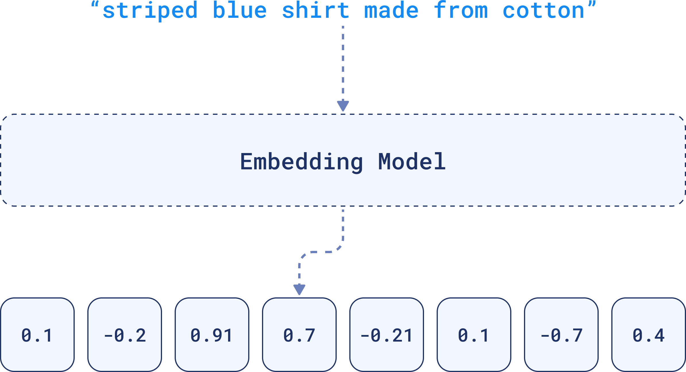
These numbers are generated by embedding models, such as deep learning algorithms, and capture the essential patterns or relationships within the data. That’s why the term embedding is often used interchangeably with vector when referring to the output of these models.
To represent textual data, for example, an embedding will encapsulate the nuances of language, such as semantics and context within its dimensions.
For that reason, when comparing two similar sentences, their embeddings will turn out to be very similar, because they have similar linguistic elements.
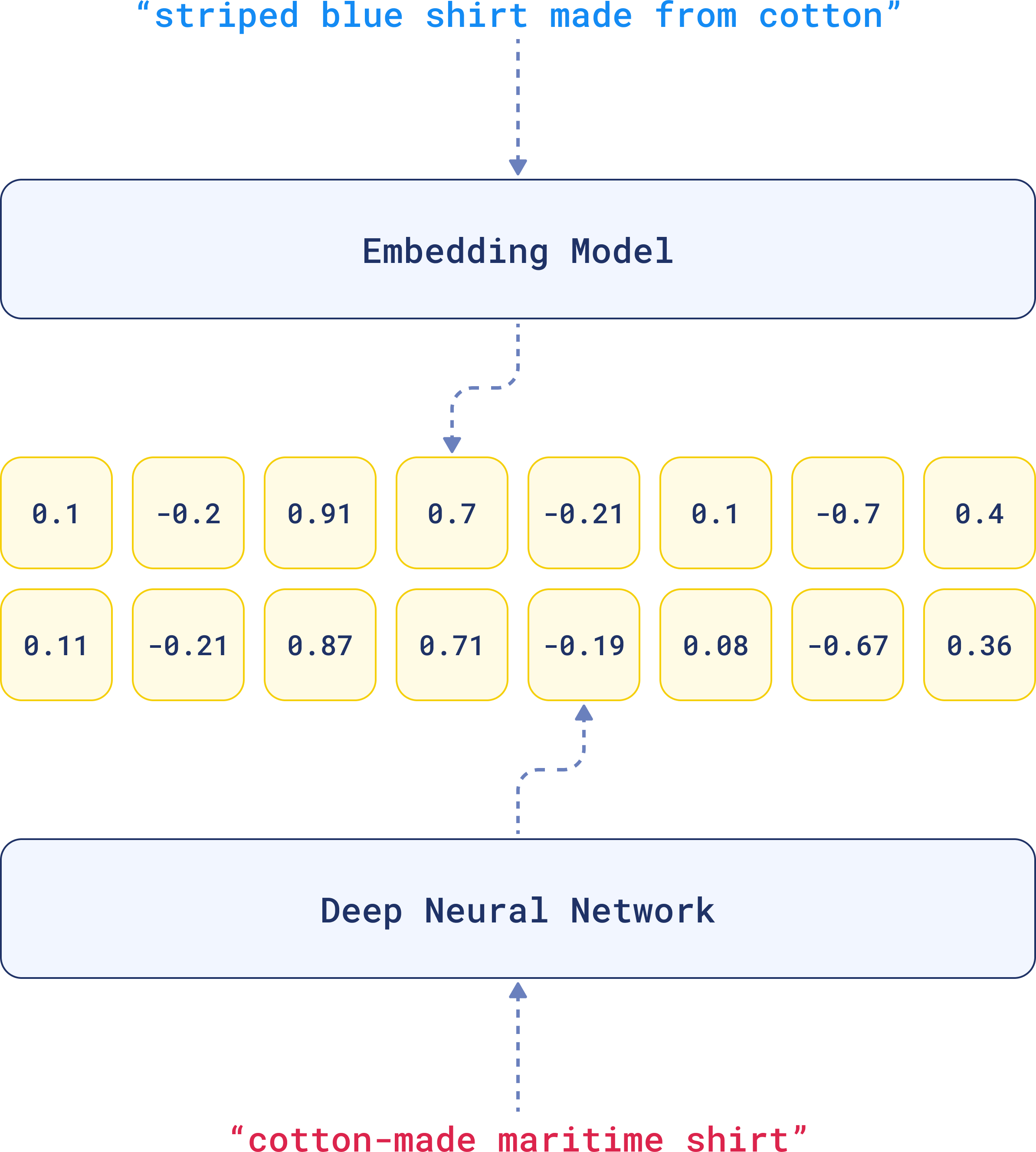
That’s the beauty of embeddings. The complexity of the data is distilled into something that can be compared across a multi-dimensional space.
3. The Payload: Adding Context with Metadata
Sometimes you’re going to need more than just numbers to fully understand or refine a search. While the dimensions capture the essence of the data, the payload holds metadata for structured information.
It could be textual data like descriptions, tags, categories, or it could be numerical values like dates or prices. This extra information is vital when you want to filter or rank search results based on criteria that aren’t directly encoded in the vector.
This metadata is invaluable when you need to apply additional filters or sorting criteria.
For example, if you’re searching for a picture of a dog, the vector helps the database find images that are visually similar. But let’s say you want results showing only images taken within the last year, or those tagged with “vacation.”
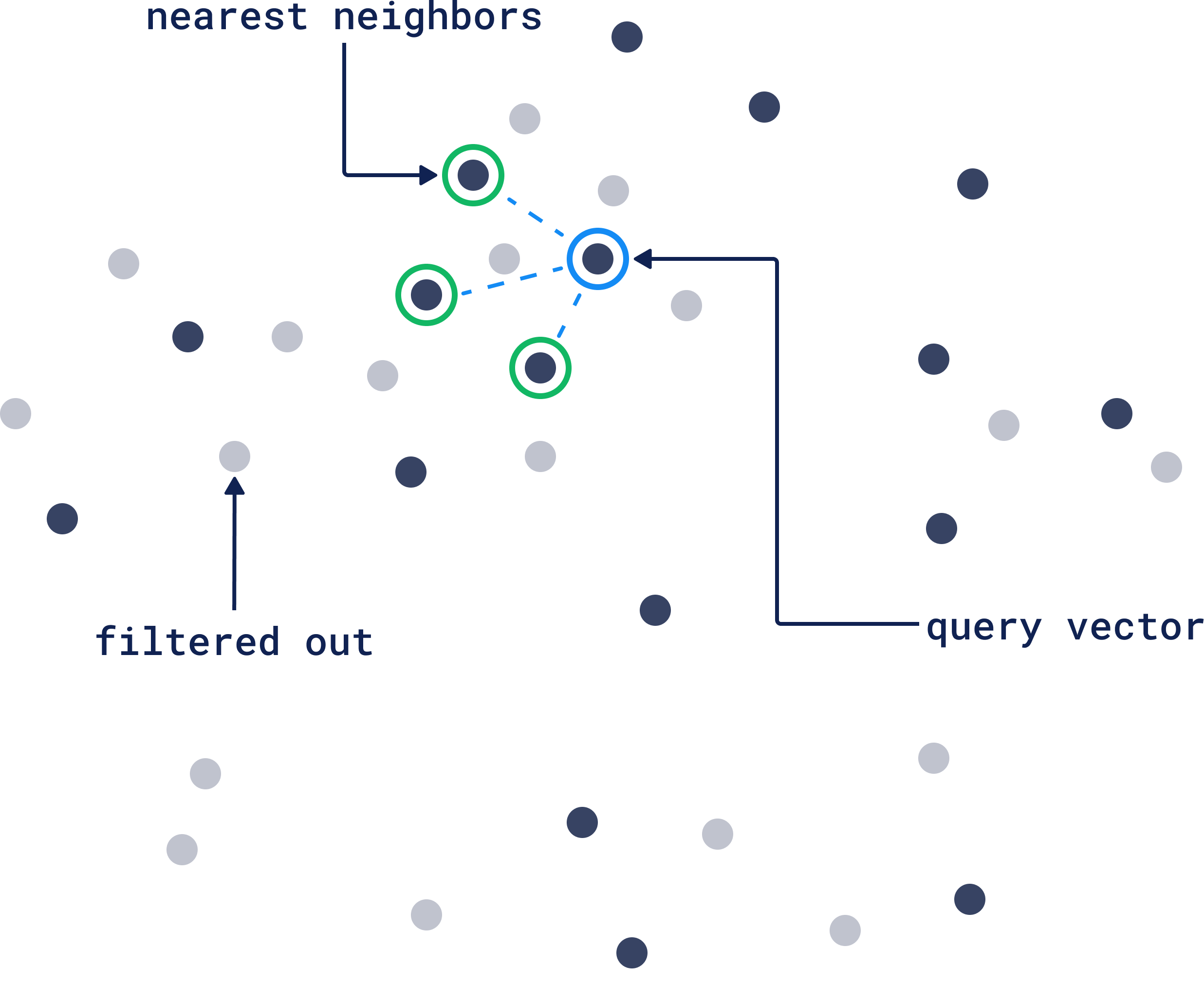
The payload can help you narrow down those results by ignoring vectors that don’t match your query vector filtering criteria. If you want the full picture of how filtering works in Qdrant, check out our Complete Guide to Filtering.
The Architecture of a Vector Database
A vector database is made of multiple different entities and relations. Let’s understand a bit of what’s happening here:
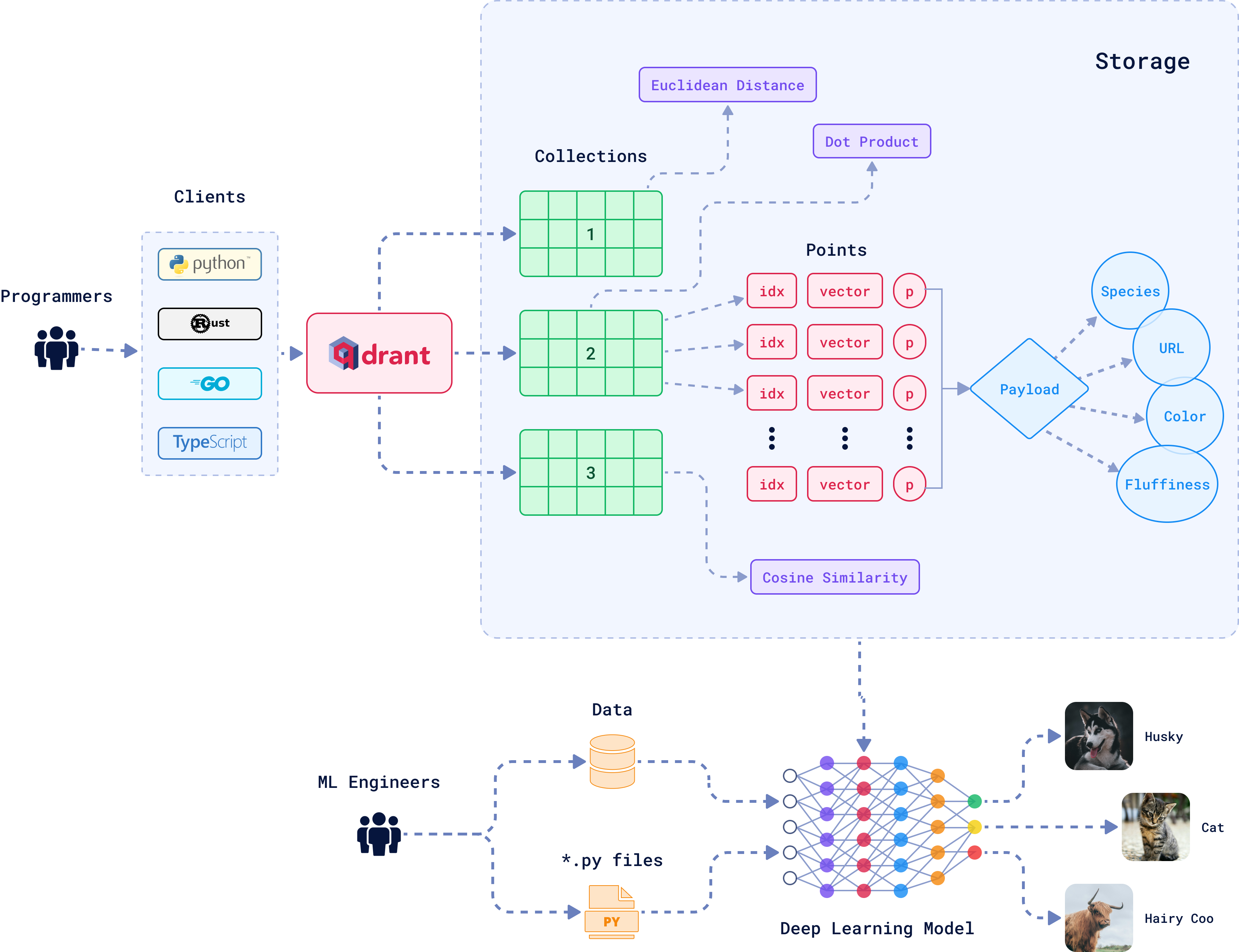
Collections
A collection is essentially a group of vectors (or “points”) that are logically grouped together based on similarity or a specific task. Every vector within a collection shares the same dimensionality and can be compared using a single metric. Avoid creating multiple collections unless necessary; instead, consider techniques like sharding for scaling across nodes or multitenancy for handling different use cases within the same infrastructure.
Distance Metrics
These metrics defines how similarity between vectors is calculated. The choice of distance metric is made when creating a collection and the right choice depends on the type of data you’re working with and how the vectors were created. Here are the three most common distance metrics:
Euclidean Distance: The straight-line path. It’s like measuring the physical distance between two points in space. Pick this one when the actual distance (like spatial data) matters.
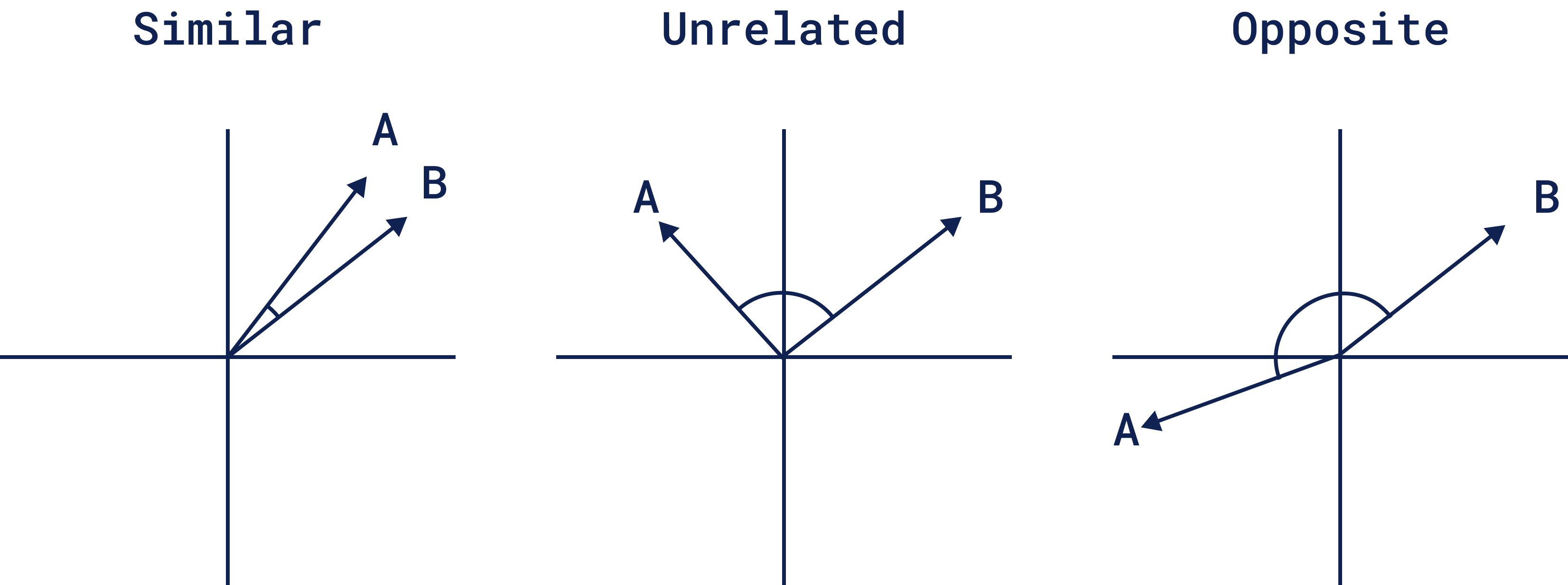
Cosine Similarity: This one is about the angle, not the length. It measures how two vectors point in the same direction, so it works well for text or documents when you care more about meaning than magnitude. For example, if two things are similar, opposite, or unrelated:
- Dot Product: This looks at how much two vectors align. It’s popular in recommendation systems where you’re interested in how much two things “agree” with each other.
RAM-Based and Memmap Storage
By default, Qdrant stores vectors in RAM, delivering incredibly fast access for datasets that fit comfortably in memory. But when your dataset exceeds RAM capacity, Qdrant offers Memmap as an alternative.
Memmap allows you to store vectors on disk, yet still access them efficiently by mapping the data directly into memory if you have enough RAM. To enable it, you only need to set "on_disk": true when you are creating a collection:
from qdrant_client import QdrantClient, models

client = QdrantClient(url='http://localhost:6333')

client.create_collection(
    collection_name="{collection_name}",
    vectors_config=models.VectorParams(
        size=768, distance=models.Distance.COSINE, on_disk=True
    ),
)
For other configurations like hnsw_config.on_disk or memmap_threshold, see the Qdrant documentation for Storage.
SDKs
Qdrant offers a range of SDKs. You can use the programming language you’re most comfortable with, whether you’re coding in Python, Go, Rust, Javascript/Typescript, C# or Java.
The Core Functionalities of Vector Databases

When you think of a traditional database, the operations are familiar: you create, read, update, and delete records. These are the fundamentals. And guess what? In many ways, vector databases work the same way, but the operations are translated for the complexity of vectors.
1. Indexing: HNSW Index and Sending Data to Qdrant
Indexing your vectors is like creating an entry in a traditional database. But for vector databases, this step is very important. Vectors need to be indexed in a way that makes them easy to search later on.
HNSW (Hierarchical Navigable Small World) is a powerful indexing algorithm that most vector databases rely on to organize vectors for fast and efficient search.
It builds a multi-layered graph, where each vector is a node and connections represent similarity. The higher layers connect broadly similar vectors, while lower layers link vectors that are closely related, making searches progressively more refined as they go deeper.
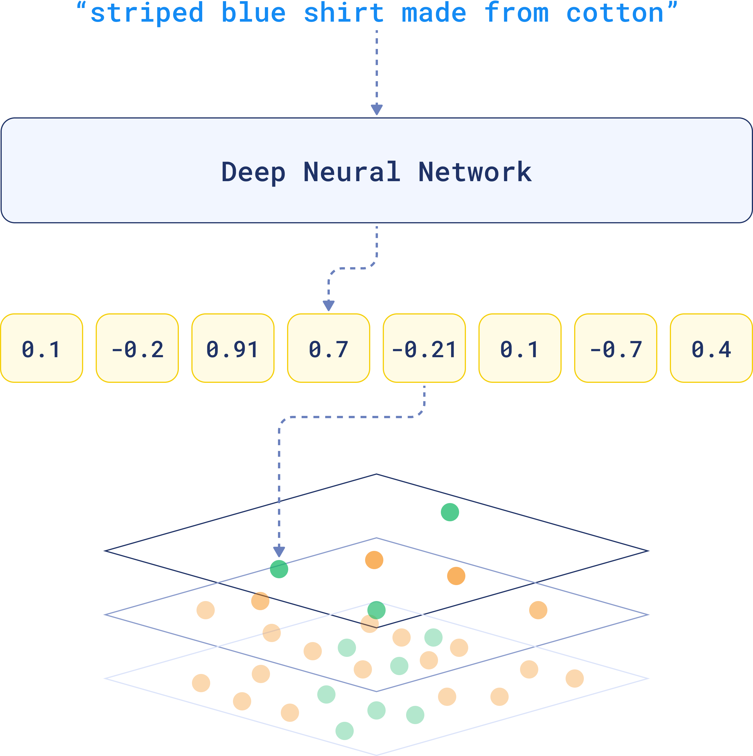
When you run a search, HNSW starts at the top, quickly narrowing down the search by hopping between layers. It focuses only on relevant vectors as it goes deeper, refining the search with each step.
1.1 Payload Indexing
In Qdrant, indexing is modular. You can configure indexes for both vectors and payloads independently. The payload index is responsible for optimizing filtering based on metadata. Each payload index is built for a specific field and allows you to quickly filter vectors based on specific conditions.
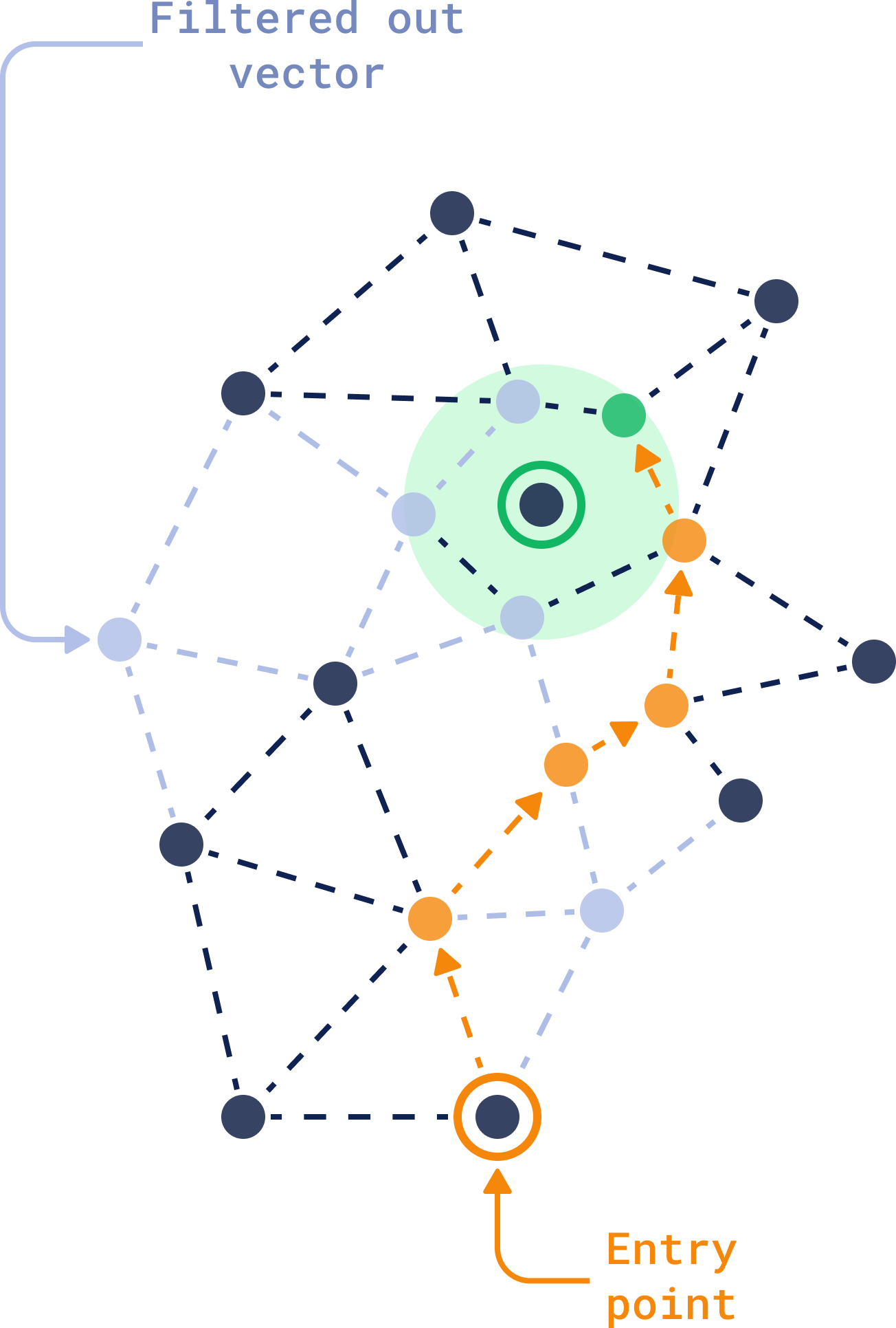
You need to build the payload index for each field you’d like to search. The magic here is in the combination: HNSW finds similar vectors, and the payload index makes sure only the ones that fit your criteria come through. Learn more about Qdrant’s Filterable HNSW and why it was built like this.
Combining full-text search with vector-based search gives you even more versatility. You can simultaneously search for conceptually similar documents while ensuring specific keywords are present, all within the same query.
2. Searching: Approximate Nearest Neighbors (ANN) Search
Similarity search allows you to search by meaning. This way you can do searches such as similar songs that evoke the same mood, finding images that match your artistic vision, or even exploring emotional patterns in text.

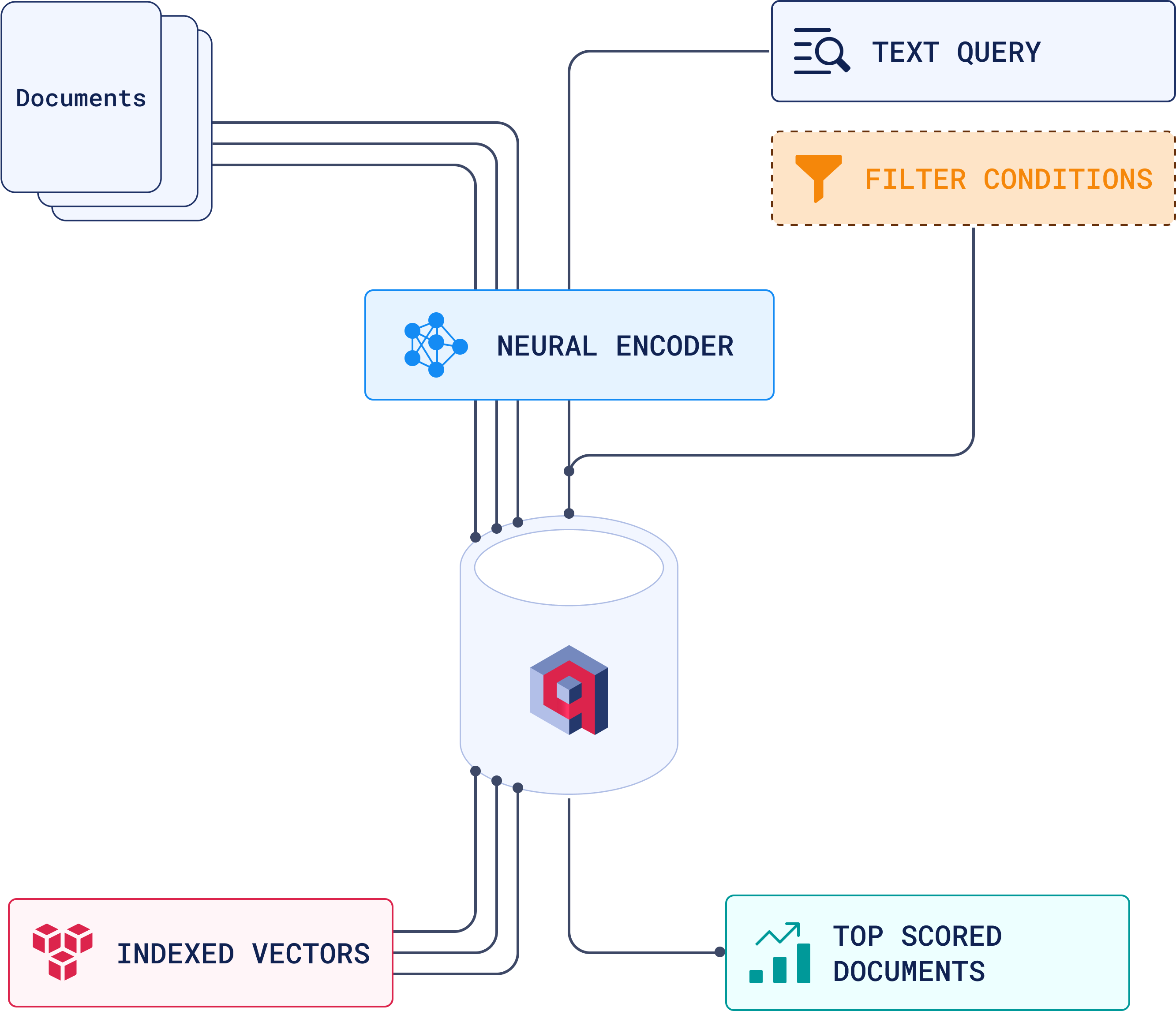
The way it works is, when the user queries the database, this query is also converted into a vector. The algorithm quickly identifies the area of the graph likely to contain vectors closest to the query vector.
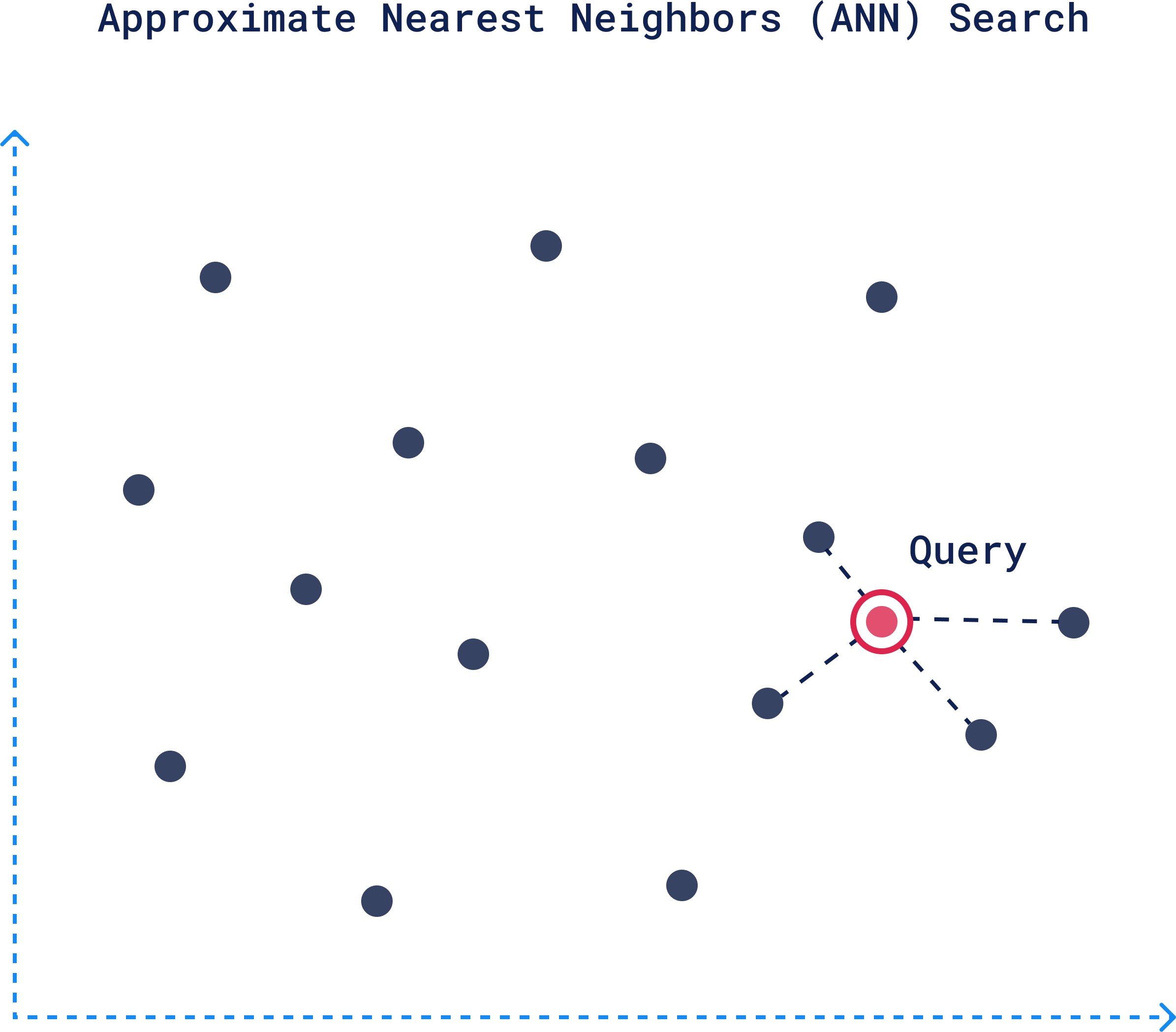
The search then moves down progressively narrowing down to more closely related and relevant vectors. Once the closest vectors are identified at the bottom layer, these points translate back to actual data, representing your top-scored documents.
Here’s a high-level overview of this process:
3. Updating Vectors: Real-Time and Bulk Adjustments
Data isn’t static, and neither are vectors. Keeping your vectors up to date is crucial for maintaining relevance in your searches.
Vector updates don’t always need to happen instantly, but when they do, Qdrant handles real-time modifications efficiently with a simple API call:
client.upsert(
    collection_name='product_collection',
    points=[PointStruct(id=product_id, vector=new_vector, payload=new_payload)]
)
For large-scale changes, like re-indexing vectors after a model update, batch updating allows you to update multiple vectors in one operation without impacting search performance:
batch_of_updates = [
    PointStruct(id=product_id_1, vector=updated_vector_1, payload=new_payload_1),
    PointStruct(id=product_id_2, vector=updated_vector_2, payload=new_payload_2),
    # Add more points...
]

client.upsert(
    collection_name='product_collection',
    points=batch_of_updates
)
4. Deleting Vectors: Managing Outdated and Duplicate Data
Efficient vector management is key to keeping your searches accurate and your database lean. Deleting vectors that represent outdated or irrelevant data, such as expired products, old news articles, or archived profiles, helps maintain both performance and relevance.
In Qdrant, removing vectors is straightforward, requiring only the vector IDs to be specified:
client.delete(
    collection_name='data_collection',
    points_selector=[point_id_1, point_id_2]
)
You can use deletion to remove outdated data, clean up duplicates, and manage the lifecycle of vectors by automatically deleting them after a set period to keep your dataset relevant and focused.
Dense vs. Sparse Vectors

Now that you understand what vectors are and how they are created, let’s learn more about the two possible types of vectors you can use: dense or sparse. The main difference between the two are:
1. Dense Vectors
Dense vectors are, quite literally, dense with information. Every element in the vector contributes to the semantic meaning, relationships and nuances of the data. A dense vector representation of this sentence might look like this:
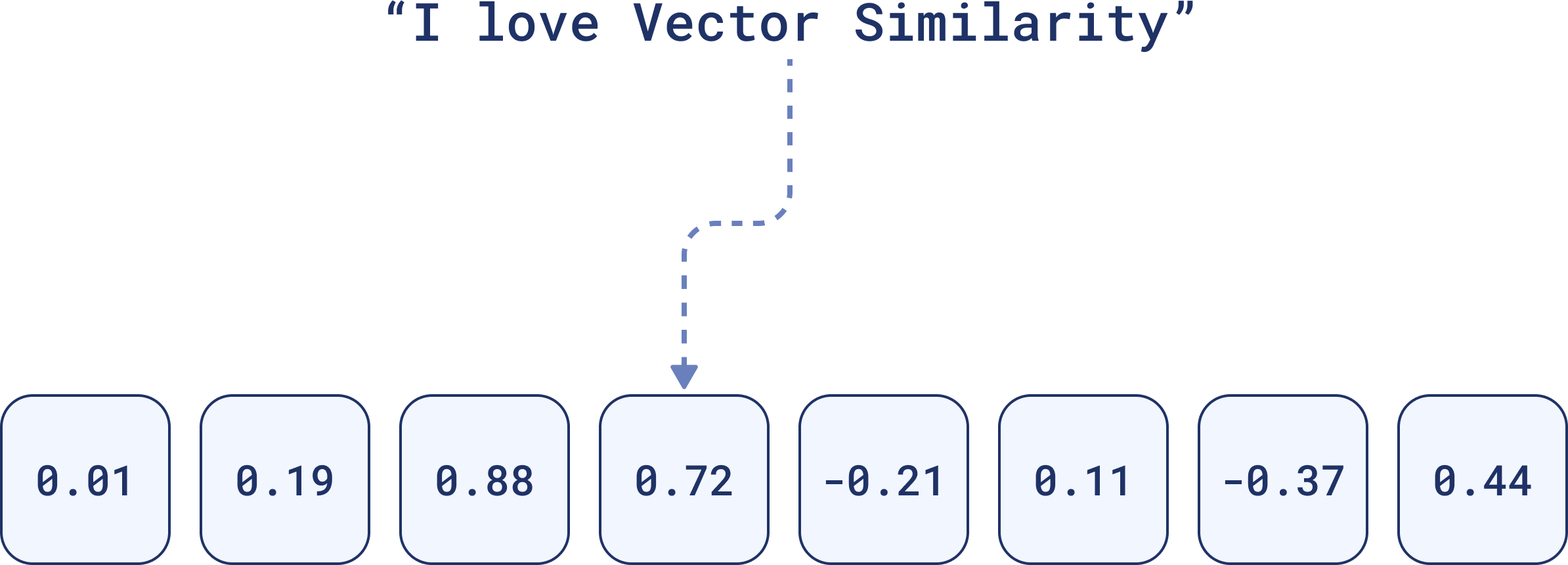
Each number holds weight. Together, they convey the overall meaning of the sentence, and are better for identifying contextually similar items, even if the words don’t match exactly.
2. Sparse Vectors
Sparse vectors operate differently. They focus only on the essentials. In most sparse vectors, a large number of elements are zeros. When a feature or token is present, it’s marked—otherwise, zero.
In the image, you can see a sentence, “I love Vector Similarity,” broken down into tokens like “i,” “love,” “vector” through tokenization. Each token is assigned a unique ID from a large vocabulary. For example, “i” becomes 193, and “vector” becomes 15012.
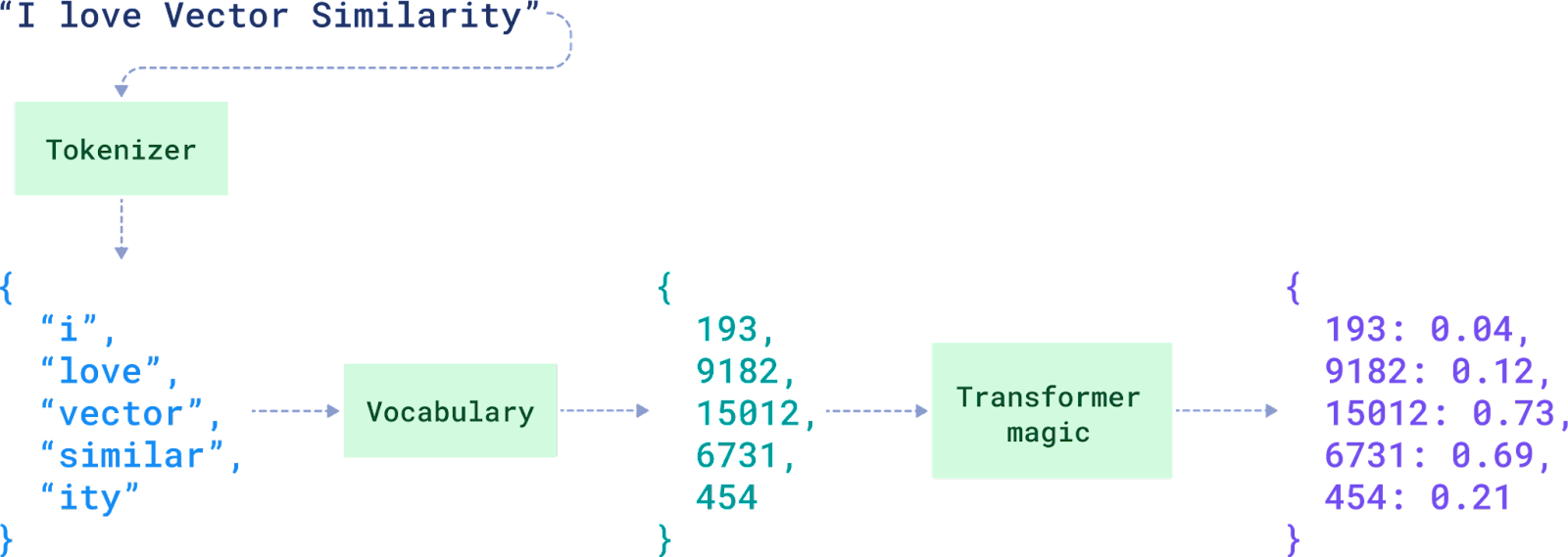
Sparse vectors, are used for exact matching and specific token-based identification. The values on the right, such as 193: 0.04 and 9182: 0.12, are the scores or weights for each token, showing how relevant or important each token is in the context. The final result is a sparse vector:
{
   193: 0.04,
   9182: 0.12,
   15012: 0.73,
   6731: 0.69,
   454: 0.21
}
Everything else in the vector space is assumed to be zero.
Sparse vectors are ideal for tasks like keyword search or metadata filtering, where you need to check for the presence of specific tokens without needing to capture the full meaning or context. They suited for exact matches within the data itself, rather than relying on external metadata, which is handled by payload filtering.
Benefits of Hybrid Search

Sometimes context alone isn’t enough. Sometimes you need precision, too. Dense vectors are fantastic when you need to retrieve results based on the context or meaning behind the data. Sparse vectors are useful when you also need keyword or specific attribute matching.
With hybrid search you don’t have to choose one over the other and use both to get searches that are more relevant and filtered.
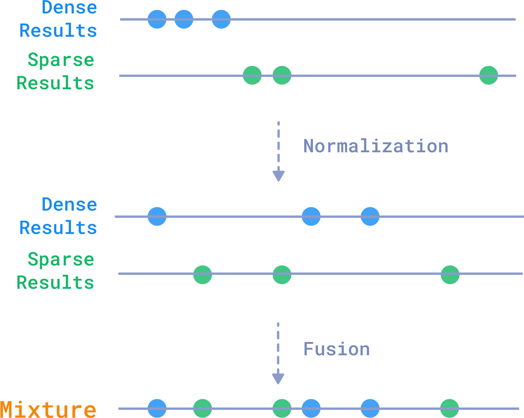
To achieve this balance, Qdrant uses normalization and fusion techniques to blend results from multiple search methods. One common approach is Reciprocal Rank Fusion (RRF), where results from different methods are merged, giving higher importance to items ranked highly by both methods. This ensures that the best candidates, whether identified through dense or sparse vectors, appear at the top of the results.
Qdrant combines dense and sparse vector results through a process of normalization and fusion.
How to Use Hybrid Search in Qdrant
Qdrant makes it easy to implement hybrid search through its Query API. Here’s how you can make it happen in your own project:

Example Hybrid Query: Let’s say a researcher is looking for papers on NLP, but the paper must specifically mention “transformers” in the content:
search_query = {
    "vector": query_vector,  # Dense vector for semantic search
    "filter": {  # Filtering for specific terms
        "must": [
            {"key": "text", "match": "transformers"}  # Exact keyword match in the paper
        ]
    }
}
In this query the dense vector search finds papers related to the broad topic of NLP and the sparse vector filtering ensures that the papers specifically mention “transformers”.
This is just a simple example and there’s so much more you can do with it. See our complete article on Hybrid Search guide to see what’s happening behind the scenes and all the possibilities when building a hybrid search system.
Quantization: Get 40x Faster Results

As your vector dataset grows larger, so do the computational demands of searching through it.
Quantized vectors are much smaller and easier to compare. With methods like Binary Quantization, you can see search speeds improve by up to 40x while memory usage decreases by 32x. Improvements that can be decisive when dealing with large datasets or needing low-latency results.
It works by converting high-dimensional vectors, which typically use 4 bytes per dimension, into binary representations, using just 1 bit per dimension. Values above zero become “1”, and everything else becomes “0”.
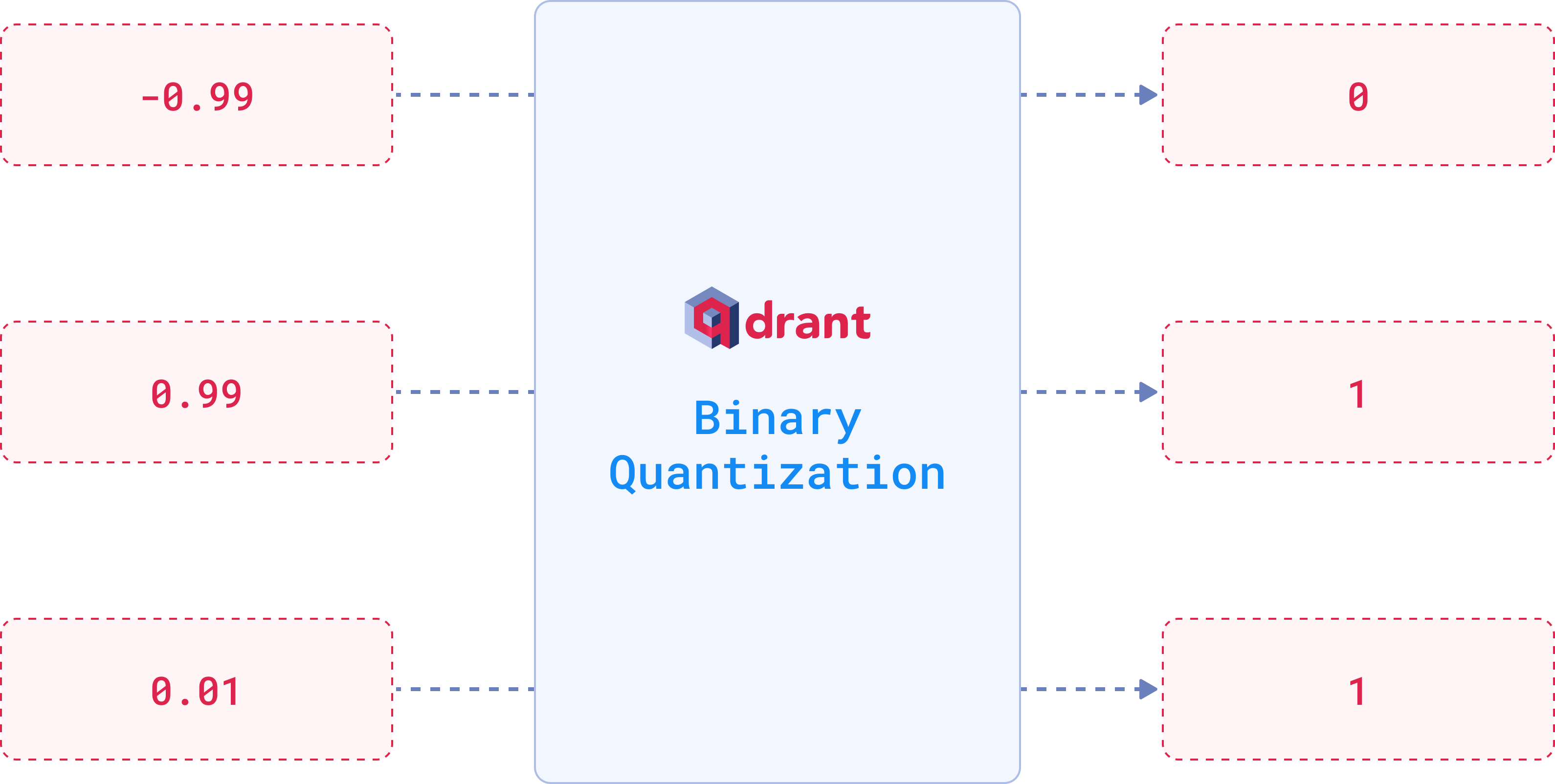
Quantization reduces data precision, and yes, this does lead to some loss of accuracy. However, for binary quantization, OpenAI embeddings achieves this performance improvement at a cost of only 5% of accuracy. If you apply techniques like oversampling and rescoring, this loss can be brought down even further.
However, binary quantization isn’t the only available option. Techniques like Scalar Quantization and Product Quantization are also popular alternatives when optimizing vector compression.
You can set up your chosen quantization method using the quantization_config parameter when creating a new collection:
client.create_collection(
    collection_name="{collection_name}",
    vectors_config=models.VectorParams(
        size=1536,
        distance=models.Distance.COSINE
    ),

    # Choose your preferred quantization method
    quantization_config=models.BinaryQuantization(
        binary=models.BinaryQuantizationConfig(
            always_ram=True,  # Store the quantized vectors in RAM for faster access
        ),
    ),
)
You can store original vectors on disk within the vectors_config by setting on_disk=True to save RAM space, while keeping quantized vectors in RAM for faster access
We recommend checking out our Vector Quantization guide for a full breakdown of methods and tips on optimizing performance for your specific use case.
Distributed Deployment
When thinking about scaling, the key factors to consider are fault tolerance, load balancing, and availability. One node, no matter how powerful, can only take you so far. Eventually, you’ll need to spread the workload across multiple machines to ensure the system remains fast and stable.
Sharding: Distributing Data Across Nodes
In a distributed Qdrant cluster, data is split into smaller units called shards, which are distributed across different nodes. which helps balance the load and ensures that queries can be processed in parallel.
Each collection—a group of related data points—can be split into non-overlapping subsets, which are then managed by different nodes.
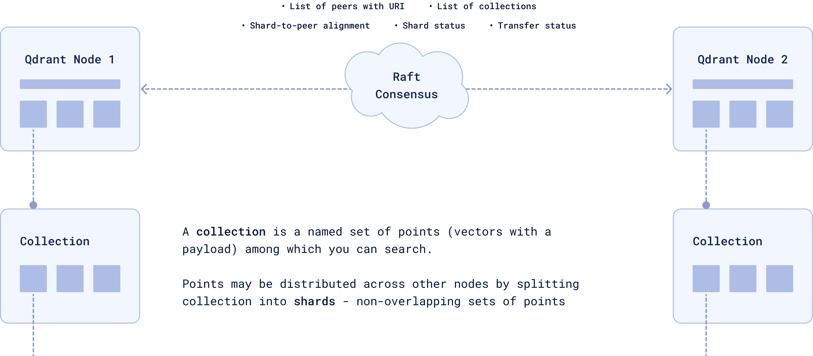
Raft Consensus ensures that all the nodes stay in sync and have a consistent view of the data. Each node knows where every shard is, and Raft ensures that all nodes are in sync. If one node fails, the others know where the missing data is located and can take over.
By default, the number of shards in your Qdrant system matches the number of nodes in your cluster. But if you need more control, you can choose the shard_number manually when creating a collection.
client.create_collection(
    collection_name="{collection_name}",
    vectors_config=models.VectorParams(size=300, distance=models.Distance.COSINE),
    shard_number=4, # Custom number of shards
)
There are two main types of sharding:
- Automatic Sharding: Points (vectors) are automatically distributed across shards using consistent hashing. Each shard contains non-overlapping subsets of the data.
- User-defined Sharding: Specify how points are distributed, enabling more control over your data organization, especially for use cases like multitenancy, where each tenant (a user, client, or organization) has their own isolated data.
Each shard is divided into segments. They are a smaller storage unit within a shard, storing a subset of vectors and their associated payloads (metadata). When a query is executed, it targets the only relevant segments, processing them in parallel.

Replication: High Availability and Data Integrity
You don’t want a single failure to take down your system, right? Replication keeps multiple copies of the same data across different nodes to ensure high availability.
In Qdrant, Replica Sets manage these copies of shards across different nodes. If one replica becomes unavailable, others are there to take over and keep the system running. Whether the data is local or remote is mainly influenced by how you’ve configured the cluster.
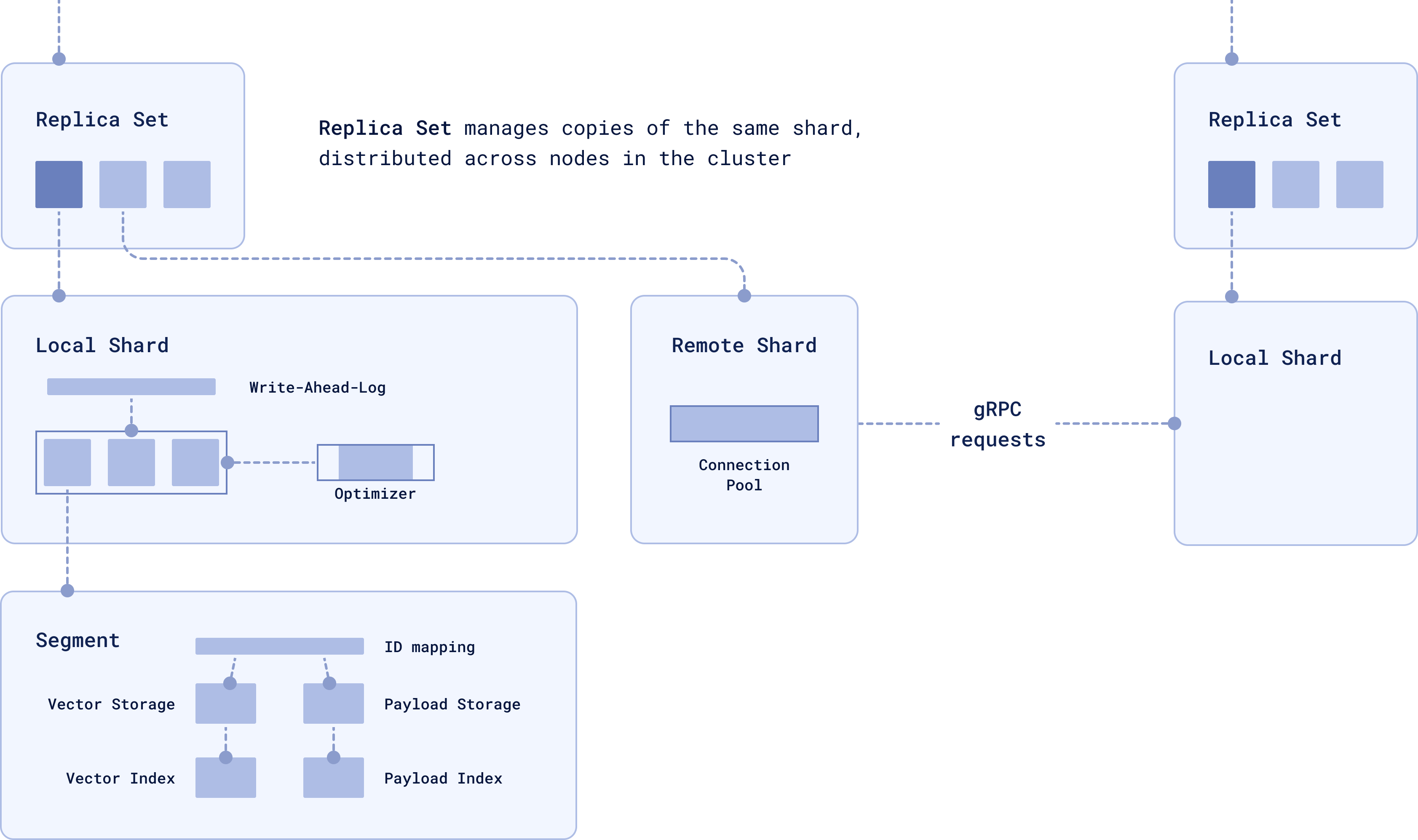
When a query is made, if the relevant data is stored locally, the local shard handles the operation. If the data is on a remote shard, it’s retrieved via gRPC.
You can control how many copies you want with the replication_factor. For example, creating a collection with 4 shards and a replication factor of 2 will result in 8 physical shards distributed across the cluster:
client.create_collection(
    collection_name="{collection_name}",
    vectors_config=models.VectorParams(size=300, distance=models.Distance.COSINE),
    shard_number=4,
    replication_factor=2,
)
We recommend using sharding and replication together so that your data is both split across nodes and replicated for availability.
For more details on features like user-defined sharding, node failure recovery, and consistency guarantees, see our guide on Distributed Deployment.
Multitenancy: Data Isolation for Multi-Tenant Architectures

Sharding efficiently distributes data across nodes, while replication guarantees redundancy and fault tolerance. But what happens when you’ve got multiple clients or user groups, and you need to keep their data isolated within the same infrastructure?
Multitenancy allows you to keep data for different tenants (users, clients, or organizations) isolated within a single cluster. Instead of creating separate collections for Tenant 1 and Tenant 2, you store their data in the same collection but tag each vector with a group_id to identify which tenant it belongs to.
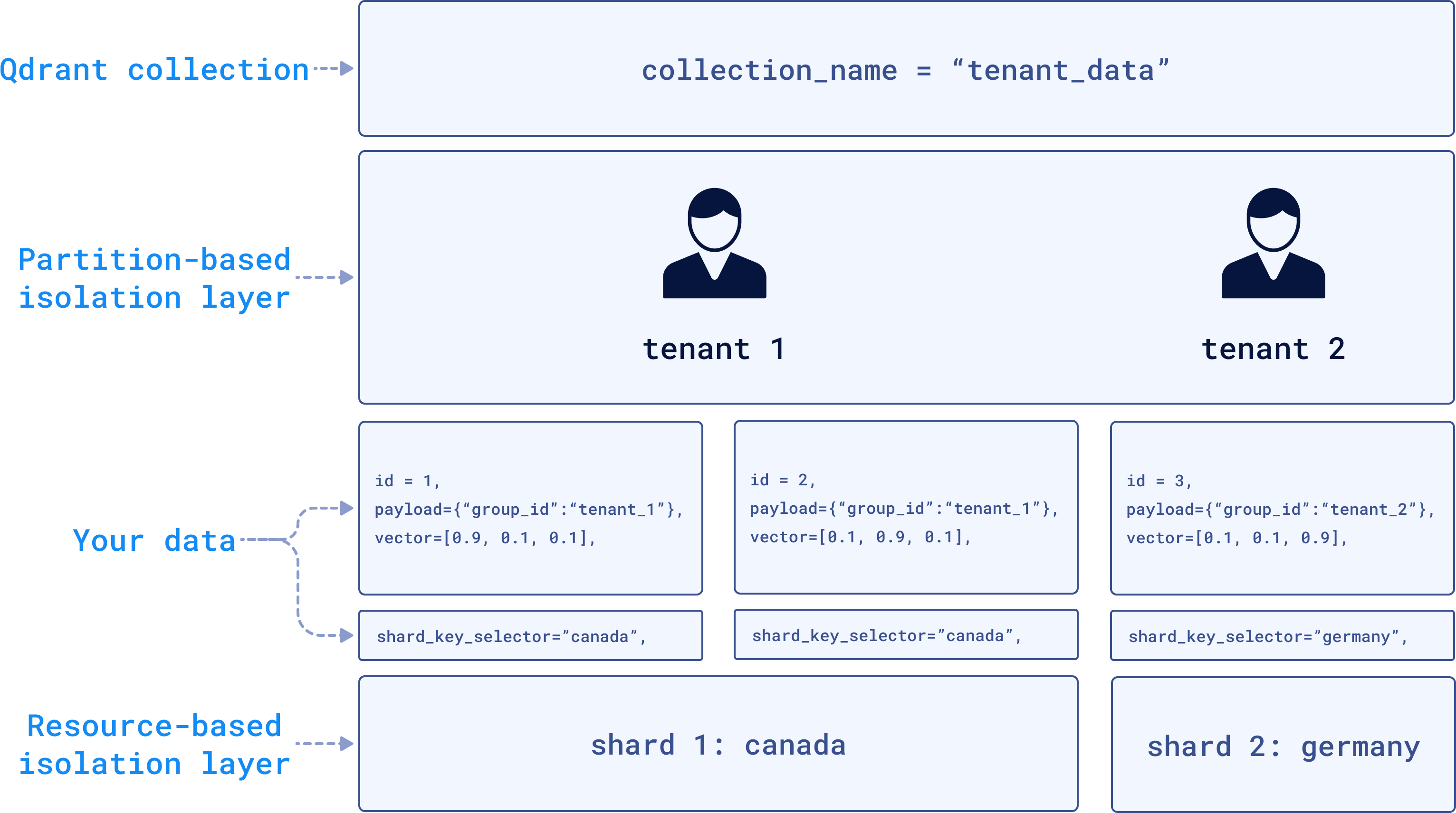
In the backend, Qdrant can store Tenant 1’s data in Shard 1 located in Canada (perhaps for compliance reasons like GDPR), while Tenant 2’s data is stored in Shard 2 located in Germany. The data will be physically separated but still within the same infrastructure.
To implement this, you tag each vector with a tenant-specific group_id during the upsert operation:
client.upsert(
    collection_name="tenant_data",
    points=[models.PointStruct(
        id=2,
        payload={"group_id": "tenant_1"},
        vector=[0.1, 0.9, 0.1]
    )],
    shard_key_selector="canada"
)
Each tenant’s data remains isolated while still benefiting from the shared infrastructure. Optimizing for data privacy, compliance with local regulations, and scalability, without the need to create excessive collections or maintain separate clusters for each tenant.
If you want to learn more about working with a multitenant setup in Qdrant, you can check out our Multitenancy and Custom Sharding dedicated guide.
Data Security and Access Control
A common security risk in vector databases is the possibility of embedding inversion attacks, where attackers could reconstruct the original data from embeddings. There are many layers of protection you can use to secure your instance that are very important before getting your vector database into production.
For quick security in simpler use cases, you can use the API key authentication. To enable it, set up the API key in the configuration or environment variable.
service:
  api_key: your_secret_api_key_here
  enable_tls: true  # Make sure to enable TLS to protect the API key from being exposed
Once this is set up, remember to include the API key in all your requests:
from qdrant_client import QdrantClient

client = QdrantClient(
    url="https://localhost:6333",
    api_key="your_secret_api_key_here"
)
In more advanced setups, Qdrant uses JWT (JSON Web Tokens) to enforce Role-Based Access Control (RBAC).
RBAC defines roles and assigns permissions, while JWT securely encodes these roles into tokens. Each request is validated against the user’s JWT, ensuring they can only access or modify data based on their assigned permissions.
You can easily setup your access tokens and secure access to sensitive data through the Qdrant Web UI:
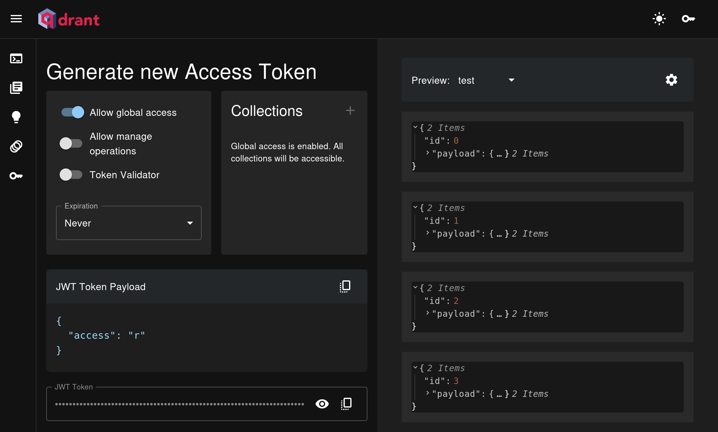
By default, Qdrant instances are unsecured, so it’s important to configure security measures before moving to production. To learn more about how to configure security for your Qdrant instance and other advanced options, please check out the official Qdrant documentation on security.
Time to Experiment
As we’ve seen in this article, a vector database is definitely not just a database as we traditionally know it. It opens up a world of possibilities, from advanced similarity search to hybrid search that allows content retrieval with both context and precision.
But there’s no better way to learn than by doing. Try building a semantic search engine or experiment deploying a hybrid search service from zero. You’ll realize there are endless ways you can take advantage of vectors.
| Use Case | How It Works | Examples |
|---|---|---|
| Similarity Search | Finds similar data points using vector distances | Find similar product images, retrieve documents based on themes, discover related topics |
| Anomaly Detection | Identifies outliers based on deviations in vector space | Detect unusual user behavior in banking, spot irregular patterns |
| Recommendation Systems | Uses vector embeddings to learn and model user preferences | Personalized movie or music recommendations, e-commerce product suggestions |
| RAG (Retrieval-Augmented Generation) | Combines vector search with large language models (LLMs) for contextually relevant answers | Customer support, auto-generate summaries of documents, research reports |
| Multimodal Search | Search across different types of data like text, images, and audio in a single query. | Search for products with a description and image, retrieve images based on audio or text |
| Voice & Audio Recognition | Uses vector representations to recognize and retrieve audio content | Speech-to-text transcription, voice-controlled smart devices, identify and categorize sounds |
| Knowledge Graph Augmentation | Links unstructured data to concepts in knowledge graphs using vectors | Link research papers to related studies, connect customer reviews to product features, organize patents by innovation trends |
You can also watch our video tutorial and get started with Qdrant to generate semantic search results and recommendations from a sample dataset.
Phew! I hope you found some of the concepts here useful. If you have any questions feel free to send them in our Discord Community where our team will be more than happy to help you out!
Remember, don’t get lost in vector space! 🚀


