Single node speed benchmark

Disclaimer

Even if we try to be objective, we are not experts in using all the existing vector databases. We develop Qdrant and try to make it stand out from the crowd. Due to that, we could have missed some important tweaks in different engines.

We tried our best, kept scrolling the docs up and down, and experimented with different configurations to get the most out of the tools. However, we believe you can do it better than us, so all benchmarks are fully open-sourced, and contributions are welcome!

Tested datasets

Our benchmark, inspired by github.com/erikbern/ann-benchmarks/, used the following datasets to test the performance of the engines on ANN Search tasks:

Hardware

In our experiments, we are not focusing on the absolute values of the metrics but rather on a relative comparison of different engines. What is important is the fact we used the same machine for all the tests. It was just wiped off between launching different engines.

We selected an average machine, which you can easily rent from almost any cloud provider. No extra quota or custom configuration is required.

For this particular experiment, we used 8 CPUs and 32GB of RAM as a Server, with additionally limited memory to 25Gb by means of Docker, to make it exact.

And 8 CPUs + 16Gb RAM for client machine. We were trying to make the bottleneck on client side as wide as possible.

Experiment setup

 ┌────────┐      ┌──────────┐
 │        ├─────►│          │
 │ Client │      │  Engine  │
 │        │◄─────┤          │
 └────────┘      └──────────┘

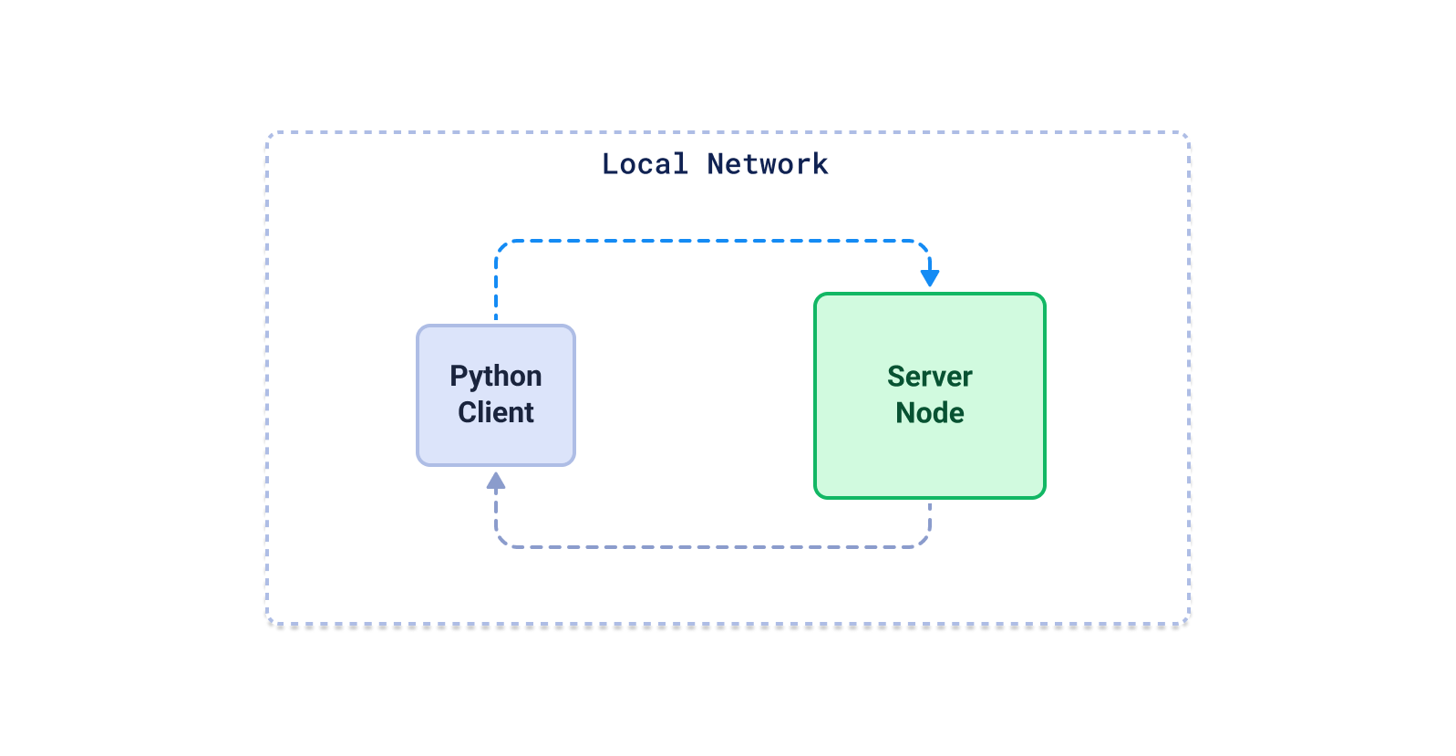
The Python Client uploads data to the server, waits for all required indexes to be constructed, and then performs searches with multiple threads. We repeat this process with multiple different configurations for each engine, and then select the best one for a given precision.

Why we decided to test with the Python client

There is no consensus in the world of vector databases when it comes to the best technology to implement such a tool. You’re free to choose Go, Java or Rust-based systems. But you’re most likely to generate your embeddings using Python with PyTorch or Tensorflow, as according to stats it is the most commonly used language for Deep Learning. Thus, you’re probably going to use Python to put the created vectors in the database of your choice either way. For that reason, using Go, Java or Rust clients will rarely happen in the typical pipeline. Python clients are also the most popular clients among all the engines, just by looking at the number of GitHub stars.

From the user’s perspective, the crucial thing is the latency perceived while using a specific library - in most cases a Python client. Nobody can and even should redefine the whole technology stack, just because of using a specific search tool. That’s why we decided to focus primarily on official Python libraries, provided by the database authors. Those may use some different protocols under the hood, but at the end of the day, we do not care how the data is transferred, as long as it ends up in the target location.

How to read the results

An interactive chart that allows you to check the results achieved by each engine under selected circumstances. First of all, you can choose the dataset, the number of search threads and the metric you want to check. Then, you can select a precision level that would be satisfactory for you. After doing all this, the table under the chart will get automatically refreshed and will only display the best results of each of the engines, with all its configuration properties. The table is sorted by the value of the selected metric (RPS / Latency / p95 latency / Index time), and the first entry is always the winner of the category 🏆

The graph displays the best configuration / result for a given precision, so it allows us to avoid visual and measurement noise.

Please note that some of the engines might not satisfy the precision criteria, if you select a really high threshold. Some of them also failed on a specific dataset, due to memory issues. That’s why the list may sometimes be incomplete and not contain all the engines.

Side notes

• Redis took over 8 hours to complete with indexing the deep-image-96-angular. That’s why we interrupted the tests and didn’t include those results.
• Weaviate was able to index the deep-image-96-angular only with the lightweight configuration under a given limitations (25Gb RAM). That’s why there are only few datapoints with low precision for this dataset and Weaviate on the plot.

Conclusions

Some of the engines are clearly doing better than others and here are some interesting findings of us:

• Qdrant and Milvus are the fastest engines when it comes to indexing time. The time they need to build internal search structures is order of magnitude lower than for the competitors.
• Qdrant achives highest RPS and lowest latencies in almost all scenarios, no matter the precision threshold and the metric we choose.
• There is a noticeable difference between engines that try to do a single HNSW index and those with multiple segments. Single-segment leads to higher RPS but lowers the precision and higher indexing time. Qdrant allows you to configure the number of segments to achieve your desired goal.
• Redis does better than the others while using one thread only. When we just use a single thread, the bottleneck might be the client, not the server, where Redis’s custom protocol gives it an advantage. But it is architecturally limited to only a single thread execution, which makes it impossible to scale vertically.
• Elasticsearch is typically way slower than all the competitors, no matter the dataset and metric.