Qdrant 1.12 - Distance Matrix, Facet Counting & On-Disk Indexing

Qdrant 1.12.0 is out! Let’s look at major new features and a few minor additions:

Distance Matrix API: Efficiently calculate pairwise distances between vectors.
GUI Data Exploration Visually navigate your dataset and analyze vector relationships.
Faceting API: Dynamically aggregate and count unique values in specific fields.

Text Index on disk: Reduce memory usage by storing text indexing data on disk.
Geo Index on disk: Offload indexed geographic data on disk for memory efficiency.

Distance Matrix API for Data Insights

Qdrant is a similarity search engine. Our mission is to give you the tools to discover and understand connections between vast amounts of semantically relevant data

The Distance Matrix API is here to lay the groundwork for such tools.

In data exploration, tasks like clustering and dimensionality reduction rely on calculating distances between data points.

Use Case: A retail company with 10,000 customers wants to segment them by purchasing behavior. Each customer is stored as a vector in Qdrant, but without a dedicated API, clustering would need 10,000 separate batch requests, making the process inefficient and costly.

You can use this API to compute a sparse matrix of distances that is optimized for large datasets. Then, you can filter through the retrieved data to find the exact vector relationships that matter.

In terms of endpoints, we offer two different formats to show results:

• Pairs are simple, intutitive and ideal for graph representation.
• Offsets are more complex, but also native when defining CSR sparse matrices.

Output - Pairs

Use the pairs endpoint to compare 10 random point pairs from your dataset:

POST /collections/{collection_name}/points/search/matrix/pairs
{
    "sample": 10,
    "limit": 2
}

Configuring the sample will retrieve a random group of 10 points to compare. The limit is the number of semantic connections between points to consider.

Qdrant will list a sparse matrix of distances between the closest pairs:

{
    "result": {
        "pairs": [
            {"a": 1, "b": 3, "score": 1.4063001},
            {"a": 1, "b": 4, "score": 1.2531},
            {"a": 2, "b": 1, "score": 1.1550001},
            {"a": 2, "b": 8, "score": 1.1359},
            {"a": 3, "b": 1, "score": 1.4063001},
            {"a": 3, "b": 4, "score": 1.2218001},
            {"a": 4, "b": 1, "score": 1.2531},
            {"a": 4, "b": 3, "score": 1.2218001},
            {"a": 5, "b": 3, "score": 0.70239997},
            {"a": 5, "b": 1, "score": 0.6146},
            {"a": 6, "b": 3, "score": 0.6353},
            {"a": 6, "b": 4, "score": 0.5093},
            {"a": 7, "b": 3, "score": 1.0990001},
            {"a": 7, "b": 1, "score": 1.0349001},
            {"a": 8, "b": 2, "score": 1.1359},
            {"a": 8, "b": 3, "score": 1.0553}
        ]
    }
}

Output - Offsets

The offsets endpoint offer another format of showing the distance between points:

POST /collections/{collection_name}/points/search/matrix/offsets
{
    "sample": 10,
    "limit": 2
}

Qdrant will return a compact representation of the distances between points in the form of row and column offsets.

Two arrays, offsets_row and offsets_col, represent the positions of non-zero distance values in the matrix. Each entry in these arrays corresponds to a pair of points with a calculated distance.

{
    "result": {
        "offsets_row": [0, 0, 1, 1, 2, 2, 3, 3, 4, 4, 5, 5, 6, 6, 7, 7],
        "offsets_col": [2, 3, 0, 7, 0, 3, 0, 2, 2, 0, 2, 3, 2, 0, 1, 2],
        "scores": [
            1.4063001, 1.2531, 1.1550001, 1.1359, 1.4063001, 
            1.2218001, 1.2531, 1.2218001, 0.70239997, 0.6146, 0.6353, 
            0.5093, 1.0990001, 1.0349001, 1.1359, 1.0553
            ],
        "ids": [1, 2, 3, 4, 5, 6, 7, 8]
    }
}

To learn more about the distance matrix, read The Distance Matrix documentation.

Distance Matrix API in the Graph UI

We are adding more visualization options to the Graph Exploration Tool, introduced in v.1.11.

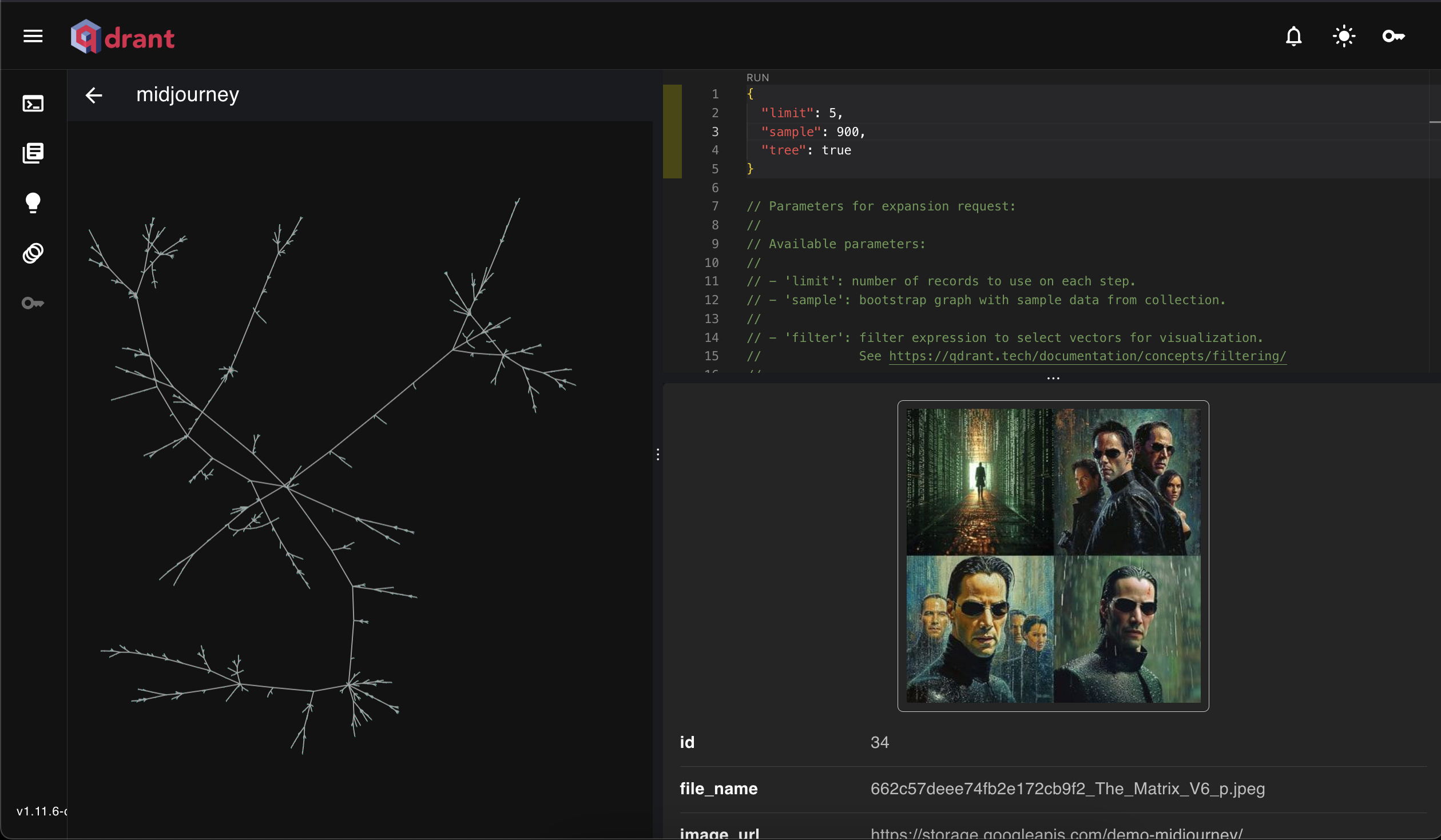
You can now leverage the Distance Matrix API from within this tool for a clearer picture of your data and its relationships.

Example: You can retrieve 900 sample points, with a limit of 5 connections per vector and a tree visualization:

{
  "limit": 5,
  "sample": 900,
  "tree": true
}

The new graphing method is cleaner and reveals relationships and outliers:

To learn more about the Web UI Dashboard, read the Interfaces documentation.

Facet API for Metadata Cardinality

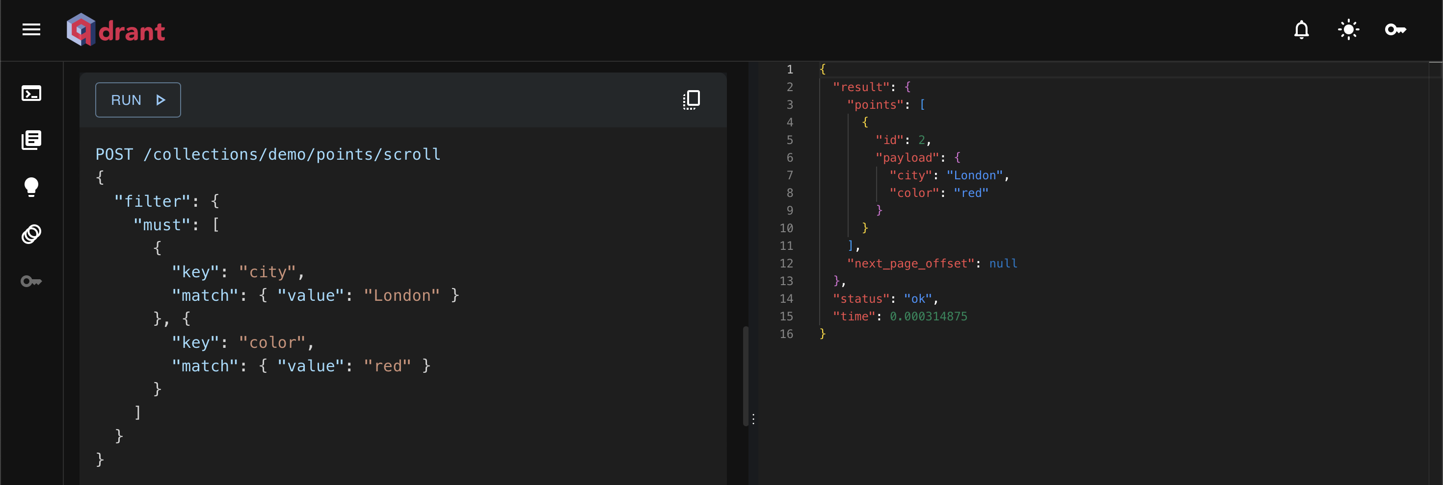
In modern applications like e-commerce, users often rely on filters, such as brand or color, to refine search results. The Facet API is designed to help users understand the distribution of values in a dataset.

The facet endpoint can efficiently count and aggregate values for a specific payload field in your dataset.

You can use it to retrieve unique values for a field, along with the number of points that contain each value. This functionality is similar to GROUP BY with COUNT(*) in SQL databases.

Note: Facet counting can only be applied to fields that support match conditions, such as fields with a keyword index.

Configuration

Here’s a sample query using the REST API to facet on the size field, filtered by products where the color is red:

POST /collections/{collection_name}/facet
{
    "key": "size",
    "filter": {
      "must": {
        "key": "color",
        "match": { "value": "red" }
      }
    }
}

This returns counts for each unique value in the size field, filtered by color = red:

{
  "response": {
    "hits": [
      {"value": "L", "count": 19},
      {"value": "S", "count": 10},
      {"value": "M", "count": 5},
      {"value": "XL", "count": 1},
      {"value": "XXL", "count": 1}
    ]
  },
  "time": 0.0001
}

The results are sorted by count in descending order and only values with non-zero counts are returned.

Configuration - Precise Facet

By default, facet counting runs an approximate filter. If you need a precise count, you can enable the exact parameter:

POST /collections/{collection_name}/facet
{
    "key": "size",
    "exact": true
}

This feature provides flexibility between performance and precision, depending on the needs of your application.

To learn more about faceting, read the Facet API documentation.

Text Index on Disk Support

Qdrant text indexing tokenizes text into smaller units (tokens) based on chosen settings (e.g., tokenizer type, token length). These tokens are stored in an inverted index for fast text searches.

With on_disk text indexing, the inverted index is stored on disk, reducing memory usage.

Configuration

Just like with other indexes, simply add on_disk: true when creating the index:

PUT /collections/{collection_name}/index
{
    "field_name": "review_text",
    "field_schema": {
        "type": "text",
        "tokenizer": "word",
        "min_token_len": 2,
        "max_token_len": 20,
        "lowercase": true,
        "on_disk": true
    }
}

To learn more about indexes, read the Indexing documentation.

Geo Index on Disk Support

For large-scale geographic datasets where storing all indexes in memory is impractical, geo indexing allows efficient filtering of points based on geographic coordinates.

With on_disk geo indexing, the index is written to disk instead of residing in memory, making it possible to handle large datasets without exhausting system memory.

This can be crucial when dealing with millions of geo points that don’t require real-time access.

Configuration

To enable this feature, modify the index schema for the geographic field by setting the on_disk: true flag.

PUT /collections/{collection_name}/index
{
    "field_name": "location",
    "field_schema": {
        "type": "geo",
        "on_disk": true
    }
}

Performance Considerations

• Cold Query Latency: On-disk indexes require I/O to load index segments, introducing slight latency on first access. Subsequent queries will benefit from disk caching.
• Hot vs. Cold Indexes: Fields frequently queried should stay in memory for faster performance, and on-disk indexes are better for large, infrequently queried fields.
• Memory vs. Disk Trade-offs: Users can manage memory by deciding which fields to store on disk.

To learn how to get the best performance from Qdrant, read the Optimization Guide.

Just the Beginning

The easiest way to reach that Hello World moment is to try vector search in a live cluster. Our interactive tutorial will show you how to create a cluster, add data and try some filtering clauses.

All of the new features from version 1.12 can be tested in the Web UI:

Check Out the Tutorial Video