Multi-Representation Search Across Titles, Abstracts, and Chunks

Time: 45 min	Level: Intermediate	Output: GitHub

A document is rarely well-represented by a single embedding. A paper has a title, an abstract, body chunks, and category tags, each carrying a different signal. Treat all four as one dense vector and the title gets averaged out; chunk-level grounding for downstream reasoning disappears.

This tutorial builds retrieval that uses each representation deliberately: named vectors per representation, fused via the Query API and grouped back to the document level for presentation.

This tutorial assumes you’ve built hybrid (dense plus sparse) search before, that you’re comfortable with named vectors, the Query API, Reciprocal Rank Fusion (RRF), and Best Matching 25 (BM25). If hybrid search is new, start with the hybrid search section of the Text Search guide first.

If you’d rather read the code, the accompanying notebook walks through this pipeline step by step with eval numbers at each stage.

Setup

Install the Python packages used throughout the tutorial:

pip install qdrant-client datasets

This tutorial uses Qdrant Cloud Inference to generate embeddings server-side. The free tier covers this tutorial's footprint. Core BM25 runs on any Qdrant instance, but dense Cloud Inference is Cloud-only. To self-host, generate dense vectors on the client with a library like FastEmbed and pass them as raw vectors instead of models.Document.

Dataset

You’ll work with 20 000 ML/CS arXiv papers (2018 and later) from the gfissore/arxiv-abstracts-2021 dataset. Each paper has a title, an abstract, and category tags, giving you three text representations once the abstract is chunked, plus categories as filterable metadata.

arXiv abstracts fit any dense model’s context window, so chunking isn’t strictly required for this dataset. We chunk anyway because the pipeline shape (chunk-level retrieval, document-level grouping) is what you’d use on full paper bodies in production. A fixed-length sentence chunker keeps the example simple; the right strategy depends on your document structure.

from datasets import load_dataset

ML_CATEGORIES = {"cs.LG", "cs.CV", "cs.CL", "cs.AI", "stat.ML"}

# Non-streaming so HF caches the parquet locally; first run downloads ~2.5 GB, re-runs are instant.
dataset = load_dataset("gfissore/arxiv-abstracts-2021", split="train")

papers = []
# IDs are roughly chronological; iterate from the end to land on 2021/2020/2019 papers first.
for i in range(len(dataset) - 1, -1, -1):
    if len(papers) >= 20000:
        break
    row = dataset[i]
    if not row["abstract"] or not row["title"]:
        continue
    # categories arrive as space-joined strings (e.g. ["cs.LG cs.CV"]); split each entry.
    cats = [tok for entry in row["categories"] for tok in entry.split()]
    if not any(c in ML_CATEGORIES for c in cats):
        continue
    # Year lives in the YYMM prefix of new-format arXiv IDs ("2104.01234" -> 2021).
    arxiv_id = row["id"]
    if "/" in arxiv_id or "." not in arxiv_id:
        continue  # skip pre-2007 IDs like "math/0506001"
    if 2000 + int(arxiv_id[:2]) < 2018:
        continue
    papers.append({
        "arxiv_id": arxiv_id,
        "title": row["title"].strip(),
        "abstract": row["abstract"].strip(),
        "tags": cats,
    })

Collection Schema

Design the collection before writing any queries. The point granularity is the chunk: every chunk of every paper becomes one point. Title and abstract embeddings are stored on every chunk so the Query API can fuse across them in a single request without an extra lookup.

from qdrant_client import QdrantClient, models

# Replace url and api_key with your own from https://cloud.qdrant.io
client = QdrantClient(
    url="https://xyz-example.qdrant.io:6333",
    api_key="<your-api-key>",
    cloud_inference=True,
)

# 384 is the output dimension of sentence-transformers/all-minilm-l6-v2, used below for every dense vector.
client.create_collection(
    collection_name="arxiv_multi_repr",
    vectors_config={
        "dense_chunk":   models.VectorParams(size=384, distance=models.Distance.COSINE),
        "dense_title":   models.VectorParams(size=384, distance=models.Distance.COSINE),
        "dense_abstract": models.VectorParams(size=384, distance=models.Distance.COSINE),
    },
    sparse_vectors_config={
        "sparse_title": models.SparseVectorParams(
            modifier=models.Modifier.IDF,
        ),
    },
)

# Index 'document_id' so the Query API can group by it; index 'tags' so we can filter on category.
client.create_payload_index(
    collection_name="arxiv_multi_repr",
    field_name="document_id",
    field_schema=models.PayloadSchemaType.KEYWORD,
)
client.create_payload_index(
    collection_name="arxiv_multi_repr",
    field_name="tags",
    field_schema=models.PayloadSchemaType.KEYWORD,
)

Each vector covers a different signal: dense_chunk for chunk content, dense_title and sparse_title for the title (dense and lexical respectively), dense_abstract for the abstract as a whole.

Categories live in the tags payload with a keyword index, so queries can pre-filter by category.

Title and abstract vectors are duplicated across every chunk of the same document. That trades storage for query simplicity: one collection, one Query API call, every representation reachable from any point. For 20 000 documents at 24 chunks each, the duplicated vectors add ~1.4 GB; storing them once per document in a sidecar collection would be ~60 MB. See Calculating RAM size for how to price this on your own corpus, and Lookup in groups to split heavy fields out and rejoin at grouping time.

Ingestion produces one point per chunk and reuses the title and abstract embeddings.

DENSE_MODEL = "sentence-transformers/all-minilm-l6-v2"
BM25_MODEL = "qdrant/bm25"

def chunk_sentences(text, target_len=2):
    """Split text into ~2-sentence chunks; fall back to the full text if it doesn't split cleanly."""
    sentences = [s.strip() for s in text.split(". ") if s.strip()]
    return [". ".join(sentences[i:i + target_len])
            for i in range(0, len(sentences), target_len)] or [text]

points = []
for paper in papers:
    chunks = chunk_sentences(paper["abstract"])

    # Title, abstract, and sparse docs are reused across every chunk of this paper; only the chunk text varies.
    # Cloud Inference embeds each Document on the server, so you don't need a client-side embedding library.
    title_doc   = models.Document(text=paper["title"],    model=DENSE_MODEL)
    abstract_doc = models.Document(text=paper["abstract"], model=DENSE_MODEL)
    # avg_len is the average word count of the indexed text.
    # Default is 256 (document-length); setting it to the actual field length (~10 here) improves BM25 scoring accuracy.
    sparse_doc  = models.Document(
        text=paper["title"],
        model=BM25_MODEL,
        options={"avg_len": 10.0},
    )

    for i, chunk in enumerate(chunks):
        points.append(models.PointStruct(
            id=len(points),
            vector={
                "dense_chunk":     models.Document(text=chunk, model=DENSE_MODEL),
                "dense_title":     title_doc,
                "dense_abstract":   abstract_doc,
                "sparse_title": sparse_doc,
            },
            payload={
                "document_id": paper["arxiv_id"],
                "title":       paper["title"],
                "tags":        paper["tags"],
                "chunk_index": i,
                "chunk_text":  chunk,
            },
        ))

client.upload_points(collection_name="arxiv_multi_repr", points=points, batch_size=256, parallel=2)

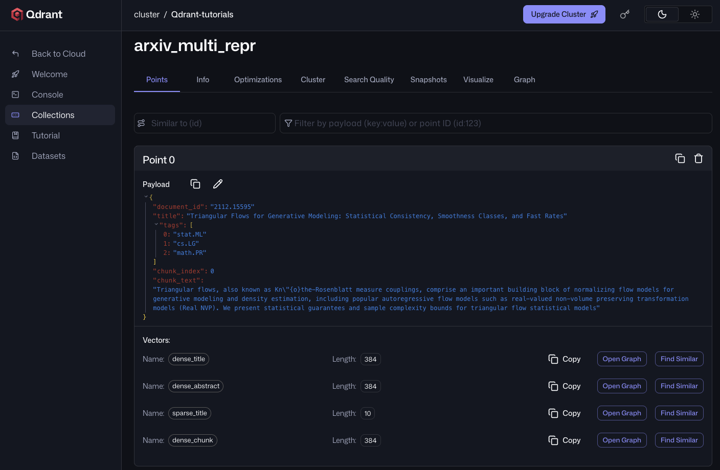
After the upload completes, opening any point in the Qdrant Cloud UI shows all four named vectors attached to one chunk. dense_chunk carries the chunk’s own embedding, while dense_title, dense_abstract, and sparse_title are the same across every chunk of this paper.

Retrieval

The recommended pipeline fuses four prefetches with Reciprocal Rank Fusion and groups the results by document. One Query API call covers retrieval, fusion, and grouping:

def retrieve(query, limit=10, group_size=3, tags=None):
    dense_query  = models.Document(text=query, model=DENSE_MODEL)
    sparse_query = models.Document(text=query, model=BM25_MODEL)
    # Optional category filter. When tags is provided, Qdrant pre-filters candidates
    # to points whose 'tags' payload includes any of the given values.
    query_filter = (
        models.Filter(must=[models.FieldCondition(key="tags", match=models.MatchAny(any=tags))])
        if tags else None
    )
    # query_points_groups runs the prefetches, fuses with RRF, applies the filter, and groups results by document_id.
    # You may need to adjust the per-prefetch limit based on the number of chunks per document; grouping only sees what the prefetch returns.
    return client.query_points_groups(
        collection_name="arxiv_multi_repr",
        prefetch=[
            models.Prefetch(query=dense_query,  using="dense_chunk",    limit=100),
            models.Prefetch(query=dense_query,  using="dense_title",    limit=100),
            models.Prefetch(query=dense_query,  using="dense_abstract", limit=100),
            models.Prefetch(query=sparse_query, using="sparse_title",   limit=100),
        ],
        query=models.FusionQuery(fusion=models.Fusion.RRF),
        query_filter=query_filter,
        group_by="document_id",
        group_size=group_size,
        limit=limit,
    ).groups

What to Prefetch

A representation only earns its own prefetch if it carries signal independent of the others. The four above are deliberately complementary:

dense_chunk carries the body content.
dense_title carries the topical naming. The title isn’t part of the chunk or abstract text in this schema, so a query matching title vocabulary that the body never repeats needs this prefetch to surface the document.
dense_abstract carries the abstract as a complete semantic unit, while dense_chunk indexes smaller sections of the document itself.
sparse_title carries lexical hits on the title that the dense embedding averages out: rare entity names, jargon, specific model or paper names.

Which Fusion to Use

Reciprocal Rank Fusion combines prefetches using document rank rather than raw scores, avoiding issues caused by dense and sparse scores operating on different scales. It’s the default configuration for this tutorial and a reasonable place to begin. In some scenarios, the variants below may produce stronger results.

For when RRF isn’t enough:

Weighted RRF. Per-prefetch weights in the rank-fusion formula. Use when one path is reliably stronger on your data; tune weights against a validation set, since a weight that helps one query class often hurts another.
Distribution-Based Score Fusion (DBSF). Normalizes each prefetch’s scores into a common range before summing. Preserves score magnitude (which RRF discards) when prefetches share a model family and score distributions are stable.
Custom formula via FormulaQuery. Full control over how scores combine:

query=models.FormulaQuery(
    formula=models.SumExpression(sum=[
        models.MultExpression(mult=[1.0, "$score[0]"]),
        models.MultExpression(mult=[0.5, "$score[1]"]),
        models.MultExpression(mult=[0.4, "$score[2]"]),
        models.MultExpression(mult=[0.3, "$score[3]"]),
    ]),
    defaults={"$score[1]": 0.0, "$score[2]": 0.0, "$score[3]": 0.0},
),

In this formula, $score[i] is the score from prefetch i, so the order of your prefetch= list matters. The defaults map provides fallback values (here 0.0) for candidates that didn’t appear in every prefetch, so the formula still evaluates.

The other two fusion strategies handle this for you: RRF discards scores entirely, and DBSF normalizes each prefetch before summing. With a custom formula, you have to normalize the scores yourself, typically using decay functions. The full FormulaQuery syntax lives in the Score Boosting reference.

For RRF vs. DBSF guidance, see the hybrid-search FAQ.

When to Boost, When to Rerank

Score boosting expresses ranking preferences that aren’t captured by retrieval scores alone: recency, source authority, geographic proximity, content type. Use a FormulaQuery whose terms reference payload fields. For time-based decay on a published_at field, use an exp_decay expression from the decay functions reference.

Use a reranker when the preference is “this is more relevant than that” but you can’t easily express why in a closed form. Formulas are cheap and deterministic; rerankers are expensive but learn what you can’t articulate.

For the step-by-step build-up that produced this design (dense baseline, plus sparse, plus title prefetch, plus grouping, plus boosting) with eval numbers showing the lift at each step, see the accompanying notebook. For a complementary view that varies the query across three representations against a single document representation, see the Universal Query for Hybrid Retrieval demo.

Wrapping Up

Multi-representation retrieval is a schema decision, not a model decision. Once each representation has its own named vector, the Query API composes them at query time: prefetch per representation, fuse with RRF, and group by document for presentation. Use a FormulaQuery or weighted fusion when you need finer control over scoring.

Real corpora rarely have clean metadata across every document. If yours has gaps and you’re unsure how to adapt this pipeline, ask in Discord. We want to hear the shape of your data.

Multi-Representation Search Across Titles, Abstracts, and Chunks

Setup

Dataset

Collection Schema

Retrieval

What to Prefetch

Which Fusion to Use

When to Boost, When to Rerank

Wrapping Up

Was this page useful?

About cookies on this site

Targeting Cookies

Functional Cookies

Strictly Necessary Cookies

Performance Cookies